Партнерка на США и Канаду по недвижимости, выплаты в крипто
- 30% recurring commission
- Выплаты в USDT
- Вывод каждую неделю
- Комиссия до 5 лет за каждого referral
The simplest method of solution of the stiff boundary value problems – the method of solution of the stiff boundary value problems without orthonormalization offered by Y. I. Vinogradov and A. Y. Vinogradov. Alexey Yurievich Vinogradov (Candidate of science /Physics and Mathematics/) (14 November 2011, Moscow, Russia) The authors: Yuri Ivanovich Vinogradov (1938 year of birth), doctor of science (Physics and Mathematics) and Alexey Yurievich Vinogradov (1970 year of birth), candidate of science (Physics and Mathematics). The idea of overcoming the problems of computing by dividing an integration interval into matching sectors belongs to Y. I. Vinogradov (doctor of science /Physics and Mathematics/). His doctorate thesis was based on that material (including that idea). Proposed realization of this idea (division and matching) through matrix theory formulas i. means of the matrix exponents (or by other words by means of a matrizant – the Cauchy matrix, Cauchy-Krylov functions) belongs to A. Y. Vinogradov (candidate of science /Physics and Mathematics/). AT PRESENT MOMENT THIS METHOD IS THE BEST ONE. The method was finalized in the mid October 2011 and a C++ software program (that is given in this paper as well) was finalized and checked by comparative computations on 14 November 2011. 1. The simplest method of solution of the stiff boundary value problems. Let’s divide a boundary value problem integration interval e. g. for three segments. We will have points (nodes) including the boundaries:
We have the boundary conditions in the following form:
We can write sector matching matrix equations as follows:
It is possible to rewrite these formulas in the more convenient form:
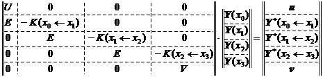
where E - unit matrix. Then in the combined matrix form we obtain a system of the linear algebraic equations in the following form:
This system is solved by the Gauss method by discrimination of the basic element. Solution in the points located between the nodes is obtained by solving the Cauchy problem with initial conditions in the ith node:
It appears to be that there is no need to apply orthonormalization for the boundary value problems for stiff ordinary differential equations. 2. Detailed description of the designations used above. Let’s use as an example a system of differential equations of the cylindrical shell of the rocket – a system of the ordinary differential equations of 8th order (after partial derivatives partitioning by the Fourier method). A system of the linear ordinary differential equations has the following form:
where The boundary conditions have the following form:
where
In case when a system of differential equations has a matrix with constant coefficients
where where Matrix exponent can be named as the Cauchy matrix or matrizant and be denoted in the following form:
Then Cauchy problem solution can be written in the following form:
where A matrix exponent (the Cauchy matrix) multiplication feature is known from the matrix theory [1]:
In case when a differential equation system has a matrix with variable coefficients
where the Cauchy matrixes are computed approximately by the following formula:
Instead of the formula for computation of the vector of the partial solution of the heterogeneous system of the differential equations in the form [1]:
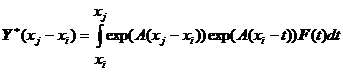
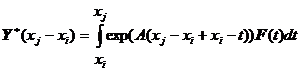
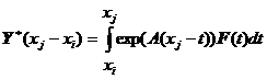
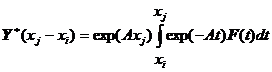
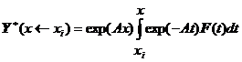
it is proposed to use the following formula for each individual segment of the integration interval:
Correctness of the above mentioned formula is justified by the following:
as was to be justified. Computation of the vector of the partial solution of the heterogeneous system of differential equations is carried out by representing the Cauchy matrix under the integral sign in the form of the series and integrating this series element by element:
This formula is correct for a system of differential equations with the constant coefficient matrix
In case of the differential equations with variable coefficients the averaged matrix Let’s consider an option when the integration interval steps are selected as sufficiently small that results in considering
It is known that at T=(at+b) we have:
In our case we have:
Then we obtain Then we obtain the series for computation of the vector of the partial solution of the heterogeneous system of differential equations in the small segment
If the segment We have We have the formula for an individual sub-segment as well:
We can write:
Let’s substitute
Let’s compare the obtained expression with the formula:
and we will obtain evidently that:
so, we obtain the formula for a particular vector:
Hence, the vectors of the sub-segments Similarly we can write
having compared this obtained expression with the formula:
we have obtained evidently that:
and at the same time we have obtained a formula for a particular vector:
Hence, a particular vector – a vector of the partial solution of the heterogeneous system of differential equations is computed by this way exactly, for example, the particular vector Computation accuracy control can be carried out by the following way. For a homogeneous system of differential equations we have:
We may write the following:
Having substituted one formula in another one we obtain:
i. e. we obtain:
however, the latter is possible only in case when
i. e. the matrixes In other words it has been proved that
i. e.
Hence, computing accuracy can be controlled by means of determination of the accuracy of matrix exponent computation (in other words the Cauchy matrixes or matrizants), that can be checked by having ascertained that the reciprocal inversion of the corresponding matrix exponents is observed in the integration segments:
putational experiments. Computational experiments have been carried out in comparison with the method of the boundary conditions transfer of Alexey Vinogradov. Line-by-line orthonormalization is used in this method. Without use of orthonormalization it is possible by means of the boundary conditions transfer method to solve a problem of cylindrical shell loading that is fixed in cantilever fashion at the right boundary and loaded at the left boundary by the force distributed uniformly by the circular arch with the ratio of the length to the radius L/R=2 and with ratio of the radius to the thickness R/h=100. In case of ratio R/h=200 the problem by means of the method of the boundary conditions transfer without orthonormalozation cannot be solved by this time because there are mistakes resulted in due to counting instability. However, in case of use of orthonormalization in the method of the boundary conditions transfer the problems related to the parameters R/h=300, R/h=500, R/h=1000 can be solved. A new method proposed in this paper allows solving of all above mentioned test problems without use of orthonormalization operation that results in significant simplification of its programming. In case of the test computations of the problems characterized by the above mentioned parameters by means of this new proposed method the integration interval is divided into 10 segments while between the nodes as aforesaid the solution was found as a solution of the Cauchy problem. 50 harmonics of the Fourier series were used for solving the problem since the result in case of usage of 50 harmonics didn’t differ from the case when 100 harmonics were used. Test problem computing speed by means of the proposed method is not less compared to the boundary conditions transfer method because both methods when used for test problems while using 50 harmonics of the Fourier series produced a final solution instantaneously after launching a program (notebook ASUS M51V CPU Duo T5800). At the same time programming of this newly proposed method is significantly simpler because there is no need in orthonormalization procedure programming. LIST OF REFERENCES 1. Gantmaher F. R. Matrix theory. – M.: Nauka, 1988. – 548 p. C++ program // sopryazhenie. cpp: main file of the project. //Solution of the boundary value problem – a cylindrical shell problem. //Integration interval is divided into 10 matching segments: left boundary – point 0 and right boundary – point 10. //WITHOUT ORTHONORMALIZATION #include "stdafx. h" #include <iostream> #include <conio. h> using namespace std; //Multiplication of A matrix by b vector and obtain rezult. void mat_on_vect(double A[8][8], double b[8], double rezult[8]){ for(int i=0;i<8;i++){ rezult[i]=0.0; for(int k=0;k<8;k++){ rezult[i]+=A[i][k]*b[k]; } } } //Computation of the matrix exponent EXP=exp(A*delta_x) void exponent(double A[8][8], double delta_x, double EXP[8][8]) { //n – number of the terms of the series in the exponent, m – a counter of the number of the terms of the series (m<=n) int n=100, m; double E[8][8]={0}, TMP1[8][8], TMP2[8][8]; int i, j,k; //E – unit matrix – the first term of the series of the exponent E[0][0]=1.0; E[1][1]=1.0; E[2][2]=1.0; E[3][3]=1.0; E[4][4]=1.0; E[5][5]=1.0; E[6][6]=1.0; E[7][7]=1.0; //initial filling-in of the auxiliary array TMP1 – the previous term of the series for follow-up multiplication //and initial filling-in of the exponent by the first term of the series for(i=0;i<8;i++) { for(j=0;j<8;j++) { TMP1[i][j]=E[i][j]; EXP[i][j]=E[i][j]; } } //series of EXP exponent computation starting from the 2nd term of the series (m=2;m<=n) for(m=2;m<=n;m++) { for(i=0;i<8;i++) { for(j=0;j<8;j++) { TMP2[i][j]=0; for(k=0;k<8;k++) { //TMP2[i][j]+=TMP1[i][k]*A[k][j]*delta_x/(m-1); TMP2[i][j]+=TMP1[i][k]*A[k][j]; } TMP2[i][j]*=delta_x;//taken out beyond the cycle of multiplication of the row by the column TMP2[i][j]/=(m-1);// taken out beyond the cycle of multiplication of the row by the column EXP[i][j]+=TMP2[i][j]; } } //filling-in of the auxiliary array TMP1 for computing the next term of the series TMP2 in the next step of the cycle by m if (m<n) { for(i=0;i<8;i++) { for(j=0;j<8;j++) { TMP1[i][j]=TMP2[i][j]; } } } } } //computation of the matrix MAT_ROW in the form of the matrix series for follow-up use //when computing a vector - partial vector – a vector of the partial solution of the heterogeneous system of the ordinary differential equations at the step delta x void mat_row_for_partial_vector(double A[8][8], double delta_x, double MAT_ROW[8][8]) { //n – number of the terms of the series in MAT_ROW, m – a counter of the number of the terms of the series (m<=n) int n=100, m; double E[8][8]={0}, TMP1[8][8], TMP2[8][8]; int i, j,k; //E – unit matrix – the first term of the series MAT_ROW E[0][0]=1.0; E[1][1]=1.0; E[2][2]=1.0; E[3][3]=1.0; E[4][4]=1.0; E[5][5]=1.0; E[6][6]=1.0; E[7][7]=1.0; //initial filling-in of the auxiliary array TMP1 – the previous term of the series for following multiplication //and initial filling-in of MAT_ROW by the first term of the series for(i=0;i<8;i++) { for(j=0;j<8;j++) { TMP1[i][j]=E[i][j]; MAT_ROW[i][j]=E[i][j]; } } //a series of computation of MAT_ROW starting from the second term of the series (m=2;m<=n) for(m=2;m<=n;m++) { for(i=0;i<8;i++) { for(j=0;j<8;j++) { TMP2[i][j]=0; for(k=0;k<8;k++) { TMP2[i][j]+=TMP1[i][k]*A[k][j]; } TMP2[i][j]*=delta_x; TMP2[i][j]/=m; MAT_ROW[i][j]+=TMP2[i][j]; } } //filling-in of the auxiliary array TMP1 for computing the next term of the series – TMP2 in the next step of the cycle by m if (m<n) { for(i=0;i<8;i++) { for(j=0;j<8;j++) { TMP1[i][j]=TMP2[i][j]; } } } } } //specifying the external influence vector in the system of ordinary differential equations – POWER vector: Y'(x)=A*Y(x)+POWER(x): void power_vector_for_partial_vector(double x, double POWER[8]){ POWER[0]=0.0; POWER[1]=0.0; POWER[2]=0.0; POWER[3]=0.0; POWER[4]=0.0; POWER[5]=0.0; POWER[6]=0.0; POWER[7]=0.0; } //computation of the vector – ZERO (particular case) vector of the partial solution //heterogeneous system of differential equations in the segment of interest: void partial_vector(double vector[8]){ for(int i=0;i<8;i++){ vector[i]=0.0; } } //computation of the vector – the vector of the partial solution of the heterogeneous system of differential equations in the segment of interest delta x: void partial_vector_real(double expo_[8][8], double mat_row[8][8], double x_, double delta_x, double vector[8]){ double POWER_[8]={0};//External influence vector on the shell double REZ[8]={0}; double REZ_2[8]={0}; power_vector_for_partial_vector(x_, POWER_);//Computing POWER_ at coordinate x_ mat_on_vect(mat_row, POWER_, REZ);//Multiplication of the matrix mat_row by POWER vector and obtain REZ vector mat_on_vect(expo_, REZ, REZ_2);// Multiplication of matrix expo_ by vector REZ and obtain vector REZ_2 for(int i=0;i<8;i++){ vector[i]=REZ_2[i]*delta_x; } } //Solution of SLAE of 88 dimensionality by the Gauss method with discrimination of the basic element int GAUSS(double AA[8*11][8*11], double bb[8*11], double x[8*11]){ double A[8*11][8*11]; double b[8*11]; for(int i=0;i<(8*11);i++){ b[i]=bb[i];//we will operate with the vector of the и right parts to provide that initial vector bb would not change when exiting the subprogram for(int j=0;j<(8*11);j++){ A[i][j]=AA[i][j];//we will operate with A matrix to provide that initial AA matrix would not change when exiting the subprogram } } int e;//number of the row where main (maximal) coefficient in the column jj is found double s, t, main;//Ancillary quantity for(int jj=0;jj<((8*11)-1);jj++){//Cycle by columns jj of transformation of A matrix into upper-triangle one e=-1; s=0.0; main=A[jj][jj]; for(int i=jj;i<(8*11);i++){//there is a number of у row where main (maximal) element is placed in the column jj and row interchanging is made if ((A[i][jj]*A[i][jj])>s) {//Instead of multiplication (potential minus sign is deleted) it could be possible to use a function by abs() module e=i; s=A[i][jj]*A[i][jj]; } } if (e<0) { cout<<"Mistake "<<jj<<"\n"; return 0; } if (e>jj) {//If the main element isn’t placed in the row with jj number but is placed in the row with у number main=A[e][jj]; for(int j=0;j<(8*11);j++){//interchanging of two rows with e and jj numbers t=A[jj][j]; A[jj][j]=A[e][j]; A[e][j]=t; } t=b[jj]; b[jj]=b[e]; b[e]=t; } for(int i=(jj+1);i<(8*11);i++){//reduction to the upper-triangle matrix for(int j=(jj+1);j<(8*11);j++){ A[i][j]=A[i][j]-(1/main)*A[jj][j]*A[i][jj];//re-calculation of the coefficients of the row i>(jj+1) } b[i]=b[i]-(1/main)*b[jj]*A[i][jj]; A[i][jj]=0.0;//nullified elements of the row under diagonal element of A matrix } }//Cycle by jj columns of transformation of A matrix into upper-triangle one x[(8*11)-1]=b[(8*11)-1]/A[(8*11)-1][(8*11)-1];//initial determination of the last element of the desired solution x (87th) for(int i=((8*11)-2);i>=0;i--){//Computation of the elements of the solution x[i] from 86th to 0th t=0; for(int j=1;j<((8*11)-i);j++){ t=t+A[i][i+j]*x[i+j]; } x[i]=(1/A[i][i])*(b[i]-t); } return 0; } int main() { int nn;//Number of the harmonic starting from the 1st (without zero one) int nn_last=50;//Number of the last harmonic double Moment[100+1]={0};//An array of the physical parameter (momentum) that is computed in each point between the boundaries double step=0.05; //step=(L/R)/100 – step size of shell computation – a step of integration interval (it should be over zero, i. e. be positive) double h_div_R;//Value of h/R h_div_R=1.0/100; double c2; c2=h_div_R*h_div_R/12;//Value of h*h/R/R/12 double nju; nju=0.3; double gamma; gamma=3./4;//The force distribution angle by the left boundary //printing to files: FILE *fp; // Open for write if( (fp = fopen( "C:/test. txt", "w" )) == NULL ) // C4996 printf( "The file 'C:/test. txt' was not opened\n" ); else printf( "The file 'C:/test. txt' was opened\n" ); for(nn=1;nn<=nn_last;nn++){ //A CYCLE BY HARMONICS STARTING FROM THE 1st HARMONIC (EXCEPT ZERO ONE) double x=0.0;//A coordinate from the left boundary – it is needed in case of heterogeneous system of the ODE for computing the particular vector FF double expo_from_minus_step[8][8]={0};//The matrix for placement of the exponent in it at the step of (0-x1) type double expo_from_plus_step[8][8]={0};// The matrix for placement of the exponent in it in the step of (x1-0) type double mat_row_for_minus_expo[8][8]={0};//the auxiliary matrix for particular vector computing when moving at step of (0-x1) type double mat_row_for_plus_expo[8][8]={0};// the auxiliary matrix for particular vector computing when moving at step of (x1-0) type double U[4][8]={0};//The matrix of the boundary conditions of the left boundary of the dimensionality 4x8 double u_[4]={0};//Dimensionality 4 vector of the external influence for the boundary conditions of the left boundary double V[4][8]={0};//The boundary conditions matrix of the right boundary of the dimensionality 4x8 double v_[4]={0};// The dimensionality 4 vector of the external influence for the boundary conditions for the right boundary double Y[100+1][8]={0};//The array of the vector-solutions of the corresponding linear algebraic equations system (in each point of the interval between the boundaries): MATRIXS*Y=VECTORS double A[8][8]={0};//Matrix of the coefficients of the system of ODE double FF[8]={0};//Vector of the particular solution of the heterogeneous ODE at the integration interval sector double Y_many[8*11]={0};// a composite vector consisting of the vectors Y(xi) in 11 points from point 0 (left boundary Y(0) to the point 10 (right boundary Y(x10)) double MATRIX_many[8*11][8*11]={0};//The matrix of the system of the linear algebraic equations double B_many[8*11]={0};// a vector of the right parts of the SLAE: MATRIX_many*Y_many=B_many double Y_vspom[8]={0};//an auxiliary vector double Y_rezult[8]={0};//an auxiliary vector double nn2,nn3,nn4,nn5,nn6,nn7,nn8;//Number of the nn harmonic raised to corresponding powers nn2=nn*nn; nn3=nn2*nn; nn4=nn2*nn2; nn5=nn4*nn; nn6=nn4*nn2; nn7=nn6*nn; nn8=nn4*nn4; //Filling-in of non-zero elements of the A matrix of the coefficients of ODE system A[0][1]=1.0; A[1][0]=(1-nju)/2*nn2; A[1][3]=-(1+nju)/2*nn; A[1][5]=-nju; A[2][3]=1.0; A[3][1]=(1+nju)/(1-nju)*nn; A[3][2]=2*nn2/(1-nju); A[3][4]=2*nn/(1-nju); A[4][5]=1.0; A[5][6]=1.0; A[6][7]=1.0; A[7][1]=-nju/c2; A[7][2]=-nn/c2; A[7][4]=-(nn4+1/c2); A[7][6]=2*nn2; //Here firstly it is necessary to make filling-in by non-zero values of the matrix and boundary conditions vector U*Y[0]=u_ (on the left) and V*Y[100]=v_ (on the right): U[0][1]=1.0; U[0][2]=nn*nju; U[0][4]=nju; u_[0]=0.0;//Force T1 at the left boundary is equal to zero U[1][0]=-(1-nju)/2*nn; U[1][3]=(1-nju)/2; U[1][5]=(1-nju)*nn*c2; u_[1]=0.0;//Force S* at the left boundary is equal to zero U[2][4]=-nju*nn2; U[2][6]=1.0; u_[2]=0;//Momentum M1 at the left boundary is equal to zero U[3][5]=(2-nju)*nn2; U[3][7]=-1.0; u_[3]=-sin(nn*gamma)/(nn*gamma);//Force Q1* at the left boundary is distributed at the angle - gamma +gamma V[0][0]=1.0; v_[0]=0.0;// The right boundary displacement u is equal to zero V[1][2]=1.0; v_[1]=0.0;//The right boundary displacement v is equal to zero V[2][4]=1.0; v_[2]=0.0;//The right boundary displacement w is equal to zero V[3][5]=1.0; v_[3]=0.0;//The right boundary rotation angle is equal to zero //Here initial filling-in of U*Y[0]=u_ и V*Y[100]=v_ terminates exponent(A,(-step*10),expo_from_minus_step);//A negative step (step value is less than zero due to direction of matrix exponent computation) //x=0.0;//the initial value of coordinate – for partial vector computation //mat_row_for_partial_vector(A, step, mat_row_for_minus_expo); //Filling-in of the SLAE coefficients matrix MATRIX_many for(int i=0;i<4;i++){ for(int j=0;j<8;j++){ MATRIX_many[i][j]=U[i][j]; MATRIX_many[8*11-4+i][8*11-8+j]=V[i][j]; } B_many[i]=u_[i]; B_many[8*11-4+i]=v_[i]; } for(int kk=0;kk<(11-1);kk++){//(11-1) unit matrix and EXPO matrix should be written into MATRIX_many for(int i=0;i<8;i++){ MATRIX_many[i+4+kk*8][i+kk*8]=1.0;//filling-in by unit matrixes for(int j=0;j<8;j++){ MATRIX_many[i+4+kk*8][j+8+kk*8]=-expo_from_minus_step[i][j];//filling-in by matrix exponents } } } //Solution of the system of linear algebraic equations GAUSS(MATRIX_many, B_many, Y_many); //Computation of the state vectors in 101 points – left point 0 and right point 100 exponent(A, step, expo_from_plus_step); for(int i=0;i<11;i++){//passing points filling-in in all 10 intervals (we will obtain points from 0 to 100) between 11 nodes for(int j=0;j<8;j++){ Y[0+i*10][j]=Y_many[j+i*8];//in 11 nodes the vectors are taken from SLAE solutions – from Y many } } for(int i=0;i<10;i++){//passing points filling-in in 10 intervals for(int j=0;j<8;j++){ Y_vspom[j]=Y[0+i*10][j];//the initial vector for ith segment, zero point, starting point of the ith segment } mat_on_vect(expo_from_plus_step, Y_vspom, Y_rezult); for(int j=0;j<8;j++){ Y[0+i*10+1][j]=Y_rezult[j];//the first point of the interval filling-in Y_vspom[j]=Y_rezult[j];//for the next step } mat_on_vect(expo_from_plus_step, Y_vspom, Y_rezult); for(int j=0;j<8;j++){ Y[0+i*10+2][j]=Y_rezult[j];//filling-in of the 2nd point of the interval Y_vspom[j]=Y_rezult[j];//for the next step } mat_on_vect(expo_from_plus_step, Y_vspom, Y_rezult); for(int j=0;j<8;j++){ Y[0+i*10+3][j]=Y_rezult[j];//filling-in of the 3rd point of the interval Y_vspom[j]=Y_rezult[j];//for the next step } mat_on_vect(expo_from_plus_step, Y_vspom, Y_rezult); for(int j=0;j<8;j++){ Y[0+i*10+4][j]=Y_rezult[j];//filing-in of the 4th point of the interval Y_vspom[j]=Y_rezult[j];//for the next step } mat_on_vect(expo_from_plus_step, Y_vspom, Y_rezult); for(int j=0;j<8;j++){ Y[0+i*10+5][j]=Y_rezult[j];// filing-in of the 5th point of the interval Y_vspom[j]=Y_rezult[j];// for the next step } mat_on_vect(expo_from_plus_step, Y_vspom, Y_rezult); for(int j=0;j<8;j++){ Y[0+i*10+6][j]=Y_rezult[j];// filing-in of the 6th point of the interval Y_vspom[j]=Y_rezult[j];// for the next step } mat_on_vect(expo_from_plus_step, Y_vspom, Y_rezult); for(int j=0;j<8;j++){ Y[0+i*10+7][j]=Y_rezult[j];// filing-in of the 7th point of the interval Y_vspom[j]=Y_rezult[j];// for the next step } mat_on_vect(expo_from_plus_step, Y_vspom, Y_rezult); for(int j=0;j<8;j++){ Y[0+i*10+8][j]=Y_rezult[j];// filing-in of the 8th point of the interval Y_vspom[j]=Y_rezult[j];// for the next step } mat_on_vect(expo_from_plus_step, Y_vspom, Y_rezult); for(int j=0;j<8;j++){ Y[0+i*10+9][j]=Y_rezult[j];// filing-in of the 9th point of the interval Y_vspom[j]=Y_rezult[j];// for the next step } } //Computation of the momentum in all points between the boundaries for(int ii=0;ii<=100;ii++){ Moment[ii]+=Y[ii][4]*(-nju*nn2)+Y[ii][6]*1.0;//Momentum M1 in the point [ii] //U[2][4]=-nju*nn2; U[2][6]=1.0; u_[2]=0;//Momentum M1 } }//CYCLE BY HARMONICS TERMINATES HERE for(int ii=0;ii<=100;ii++){ fprintf(fp,"%f\n",Moment[ii]); } fclose(fp); printf( "PRESS any key to continue...\n" ); _getch(); return 0; } Alexey Yurievich Vinogradov
My web-sites related to stiff boundary value problems solution methods: www. vinogradov-design. *****/math. html www. vinogradov-best. ***** www. AlexeiVinogradov. ***** www. VinogradovAlexei. ***** www. Vinogradov-Alexei. ***** www. Vinogradov-Math. ***** |
 .
.







 - an unknown vector-function of the 8x1 dimensionality problem,
  - a derivative of the unknown vector-function of 8x1 dimensionality,
  - a square matrix of the coefficients of the differential equation of 8x8 dimensionality,
  - a vector-function of the external influence on the system of 8x1 dimensionality.
 - is the value of the unknown vector-function at the left boundary x=0 of the 8x1 dimensionality,
  - a square horizontal matrix of the coefficients of the boundary conditions of the left boundary of the 4x8 dimensionality, and
  - an external influence on the left boundary of the 4x1 dimensionality.
 is the value of the unknown vector-function at the right boundary x=1 of the 8x1 dimensionality,
  - a square horizontal matrix of the coefficients of the boundary conditions of the right boundary of the 4x8 dimensionality, and
  - an external influence on the left boundary of the 4x1 dimensionality.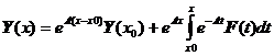
 ,
, is a unit matrix.

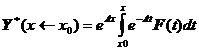 is a vector of the partial solution of the heterogeneous system of the differential equations.
 it is offered to find a solution of the Cauchy problem by means of the Cauchy matrix multiplication feature. That is the integration integral is split into small segments and the Cauchy matrixes are computed approximately in these small segments by means of the formula for a constant matrix in the exponent. Then the Cauchy matrixes computed in these small sections are multiplied:
 where
where 

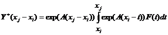
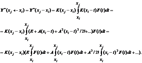
 vector can be considered in the segment
  approximately in the form of the constant value
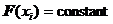 that allows its taking off from the integral sign that results in very simple series for computation in the considered segment.
 of the coefficients of the differential equation system can be used in the above mentioned formula for each segment.


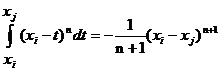 .
.
 ,
, .
. in
in  and obtain the following:




 are not added to each other simply but they are added with involvement of the Cauchy matrix of the sub-segment.
 and having substituted the formula for



 is computed similarly in the considered segment
  through the computed particular vectors
  ,
,  , and
, and  of the corresponding subs-segments
  ,
,  and
and  .
. .
. and
and
 ,
, ,
, - unit matrix,
 and
and  are inverse ones.
 .
.