Learning Asymmetry Effect for the Neuron Net Control Systems

Learning Asymmetry Effect for the Neuron Net Control Systems

Astapkovitch A. M.

Head of Student Design Center, State University of Aerospace Instrumentation

190000 Bolshaij Morskaij, 67,Saint-Petersburg, Russia

{*****@***ru}

http://www. *****

Abstract. The benchmark model of the differential drive mobile robot SOFA-2009 with the neuron net control system is described. Results of the supervised learning for different cases were compared for “moving to prescribed point of 2D surface” robot behavior under the control of two channel neuron net system. It was shown that the learning asymmetry effect exist for this type of behavior. Effect results in the asymmetry of the weight values of the symmetry control channels.

It was shown, that to avoid this effect the symmetrical learning set has to be used. One step learning procedure on base of Lagrange multipliers method is proposed, that provide possibility to take into account the existence of the linear relations for weights and avoid asymmetry effects also.

Key words: two wheel robot, benchmark model SOFA-2009, supervised learning, learning asymmetry effect, modified one step learning procedure, Lagrange multipliers method, computational robotics

Introduction

Computational Robotics methodology is supposed that the virtual robot models and the virtual environment models are used for research purposes.

SOFA-2009 is as simple as possible benchmark model of the two wheels differential drive mobile robot developed to support the student research project Phoenix-3 [1],[2]. The model reflects the most important features of the two wheels robot and consists from seven ordinary differential equations and includes description of the robot cinematic, dynamic, gears and motors.

For numerical experiments, described in this article, SOFA-2009 model was added with simplified neuron net control system. “Movement to prescribed point with slowing down” behavior was investigated. The one step supervised learning procedure was used, described in the details [3],[4]. In fact, it was shown, that very simple neuron net can be learned to solve optimal control problem of movement on 2D surface to prescribed position.

The results of learning for different samples have been compared and the existence of the learning asymmetry effect was demonstrated. This effect means that weights for two channel neuron net controller with ideal symmetry, received after supervised learning, will differ, if the asymmetry learning set was used.

It was shown also, that that symmetry solution could be received if the modified one step learning procedure is used, that takes into account the linear relations for weights. The proposed learning procedure implements the Lagrange multipliers method and it is the universal tool of the neuron net theory development.

1.  Benchmark Robot Model SOFA –2009

SOFA is a virtual two wheels differential drive mobile robot. Every wheel is a rigid body disk with diameter Dw. Distance between wheels is Lr and motors, gears, battery and control system are inside this space. Each wheel is driven independently with own motor. Motors have identical electromechanical structure. Robot forward/back motion is produced by both wheels been driven at the same rate. Turning is achieved by rotating the wheels with different rates.

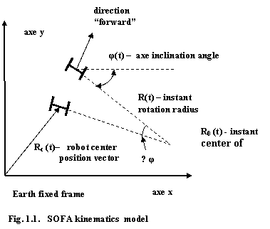
SOFA kinematic model is illustrated by fig.1.1. At any given moment of the time SOFA moving is an arc with center at the R0(t). The position of the robot center is described with vector Rc (t) and angle φ(t), that is the robot axe inclination angle, measured from the axe x.

Robot movement is described with three ordinary differential equations concluded from basic assumption of SOFA model:

φ (t+∆t)- φ (t) = ∆ φ (for left wheel) = ∆ φ (for right wheel) (1.1)

R0 (t) = R0 (t+∆t) (1.2)

Whole model is described with system of 7 ordinary differential equations (1.3-1.9). Gear for every wheel is described with equations 1.6 and 1. 7 with free parameters - k 12 , k21 Model takes into account moment of inertia of wheel Jr. Coefficients k 11 , k21 were introduced to provide flexibility to SOFA model.

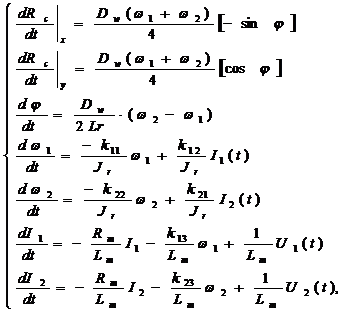(1.3-1.9)

Model SOFA-2009 is defined with parameters set : Dw = 0.3 , Lr = 0.5, Jr = 0.25,

k11 = k22 = 75 , k12= k21 = 10, Lm = 0.01, Rm = 0.1, k13= k23 = 1.5 abs(Vmax )=12 .

axe y

axe x

SOFA-2009 model was realized and verified with Mathcad 14. The ODE solver function Rkadapt (.,.,) was used for robot dynamic simulation.

2. Simplified Neuron Net Control System

To have the virtual robot valuable the model of the control system has to be added. The model depends on the research task. The simple two channels neuron net control system will be considered in this part.

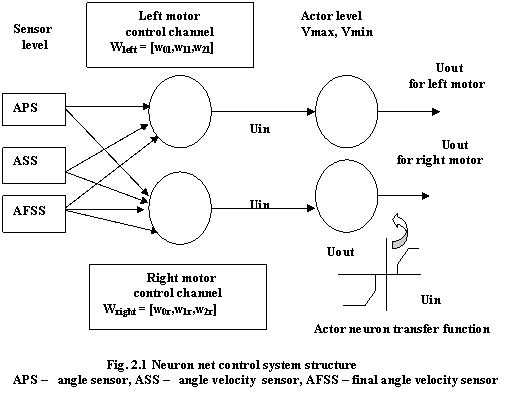
Structure of the neuron net control system is presented in fig.2.1. This system has 3 sensors and regulates the robot axe inclination angle. This system was learned to rotate robot on prescribed angle p/4 and slow down at final point with the one step supervised learning procedure [ 3]. Learning means that 6 weights (3 for every channel) have to be calculated.

Supervised learning procedure includes three steps: learning set establishing, weights calculation, control system quality estimates. The last step is the simulation of robot dynamic under neuron net control for different angle.

The same robot model SOFA-2009 was used for all steps with control system that are different for 1 and 3 steps.

The same robot model SOFA-2009 was used for all steps with control system that are different for 1 and 2, 3 steps.

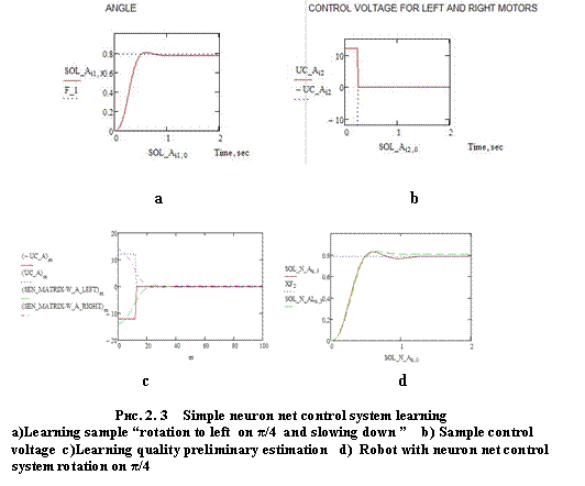
During learning set establishing, the control voltage graphs have to be created ”by hand”. To get rotation behavior left and right motors have to rotate in different directions with the same speed. For angle as large as p/4 it is naturally to use the maximal voltages VMAX and the voltages applied to left and right motors have the different signs. Duration of pulses was selected iteratively in such way that wheels rotation speed have to be 0 when angle is reaching p/4. Control voltage graphs are presented by fig. 2.3(a) and graph 2.3(b) presents the robot behavior under such type of “virtual operator” control.

During second step the variant of the one step learning procedure in one channel approximation is used.

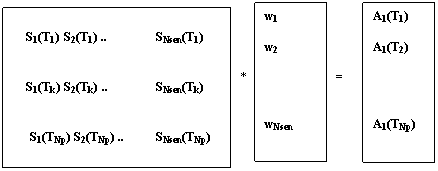
One step learning procedure is interpreted as task of the approximation for graph that is described as

 

(2.1)

where Si(Tk) – i-sensor measurements at time moment Tk, Nsen – number of sensor, Am(Tk) - sample control voltage for m -actor at time moment Tk , wi - weight of the i-sensor, Np – number of time points in learning sample

More complex possibilities of the one step learning procedure, included nonlinear approximations, are described in details in [ 3].

In matrix form system (2.1) is expressed as

S w = Ua (2.2)

where S – rectangular matrix of sensor measurements Np* Nsen, w – weights vector with dimension Nsen, Ua – the learning sample control voltage vector has dimension Np.

In described example the two channels system is used and (2.2) has to be solved twice for different control voltage samples (left and right motors) and the same sensor matrix. In common case system (2.2) is the singular one. So, to get correct solution in accordance with Adamar definition the Tichonov regularization procedure has to be used [5].

Regularization procedure can be interpreted as linear programming problem for function F(w) of neuron net weights

min F(w) = (Sw - Ua, Sw – Ua) + g (w, w) (2.3)

w

where g -is regularization coefficient, that has a small value.

In this case learning procedure is the solution of the linear equations system and the weights can be calculated with expression

w = (ST S + g E) –1 ST Ua

where E – the units square matrix with dimension Nsen*Nsen .

Some results of the described example are presented in fig. 2.3. Three sensors were used (Nsen=3): sensor of difference between robot inclination angle at final point and current one, sensor of instant angler velocity and sensor of difference of prescribed angle velocity at final point and instant one. One hundred time point was used to form the learning sample (Np =100).

Results of the learning :

·  weight vector for left channel Wt = [ 17.5 , 0.5, -0.5] ;

·  weight vector for right channel Wt = [ -17.5, - 0.5, 0.5].

Absolute values of the measurement are the same for second and third sensor, because it is supposed that at final point the angle velocity equal 0. So, learning procedure gives the same absolute value for those weights. In additional, every channel of control system has the identical parameters, so absolute values for the corresponding weights of different channel have to be the same in sense of the absolute value.

Results of preliminary estimation of the learning are presented at fig. 2.3 (с). For estimation the matrix S was multiplied by weight vector for every channel to get a voltage that will be applied to motors. As it can be seen the calculated voltage accedes the maximal accumulator voltage VMAX.

To overcome this situation the actor neurons were introduced to control net structure as it can be seen from fig. 2.1. The actor neuron imposes limits on the output voltage that depends on parameters Vmax and Vmin.

Fig 2.3 d) presents the results of simulation of robot rotation for the angle π/4 (the same value that was used for learning), under neuron net control with and without actor neuron. In the last case the actor neuron limits were Vmax =12V and Vmin =0V.

 

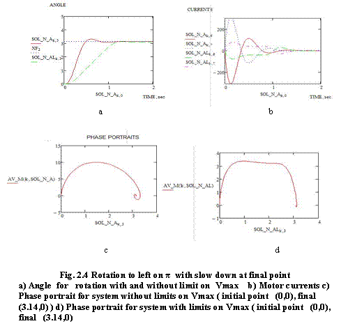
Third step is the estimation of quality of learning and the rotation for angle that differs from learning sample value. The rotation under neuron net control on the angle π is presented by fig. 2.4. The rotations were simulated for case s with and without voltage limits.

As it can be seen from presented graphs neuron net can solve this problem and robot reaches the prescribed point in the phase space. Under limits on maximal voltage robot have accelerated during initial phase and have slowed down during final one.

From this simple example of the learning some conclusion can be made. Certainly, actor neuron is a solution, but universal approach has to include description of such type limits in learning procedure.

Examples of the numerical experiments with SOFA-2009 model are described in [ 1],[2 ] and can be found on the site [6].

 

 

3. Learning Asymmetry Effect

The described above approach was used to investigate the simple neuron net control system of the robot SOFA-2009, that has to be learned to reach the prescribed point of 2D plane. The robot control system has the same structure as it presented in Fig.2.1, but number of sensors is increased up to 9. Every channel uses the same sensor set, that are described with table 3.1.

Table 3.1

Sensor description table

Name	Sensor description
DF	Distance to final point robot center position from instant position D(F)-D(Rc(t))
DV	Instant linear velocity (w1(t)+ w2(t))/2
AF	Difference between the robot inclination angle at the final point and the instant one φ (F)- φ (t)
AV	Instant robot axe inclination angle rotation speed Dw/2*Lr*( w2(t)- w1(t))
AVF	Difference between the robot angle speed at the final point and the instant one d φ - Dw/2*Lr*( w2(t)- w1(t)) dt ( F)
W1	Instant rotation speed for left wheel w1(t)
W1F	Difference between rotation speed at the final point for left wheel and the instant one w1(F)- w1(t)
W2	Instant rotation speed for right wheel w2(t)
W2F	Difference between rotation speed at the final point for right wheel and the instant one w2(F)- w1(t)

Note: F denotes the final point and D (*) is a function that calculates the distance from instant point to start one

In table 3.2 the weights for left and right channel are presented. The weights are results of the learning with the different learning samples. The initial position of the robot was the same for different learning samples, namely, robot is motionless at point (0,0) and is looking forward along axe Y (axe inclinations angle between robot axe and axe X is 0).

First two samples were used to for learning to simple behavior: rotation to left and moving forward. Third, forth and fifth samples were used to learn for more complex behavior – to reach the prescribed point of 2D plane where robot has to be slowed down and has the prescribed angle.

The presented in table 3.2 table data for sample 3 demonstrates the existence of the learning asymmetry effect. The effect leads to situation that asymmetry of learning sample is translated to weights. Because the virtual robot has the symmetrical control channels then a difference in the weights means that the reason is the learning sample asymmetry. It means that robot behavior will differ for moving to points that are situated in left and in the right half planes.

Table 3.2

Weights for different learning samples

	S C	DF	DV	AF	AV	AVF	W1	W1F	W2	W2F
1	L R	0.0 0.0	0.0 0.0	-17.5 17.5	0.093 -0.093	-0.093 0.093	-0.155 0.155	0.155 - 0.155	0.155 - 0.155	-0.155 0.155
2	L R	0.59 0.59	0. 382 0. 382	0.0 0.0	0.0 0.0	0.0 0.0	0. 382 0. 382		0. 382 0. 382
3	L R	0.239 0.251	0. 422 0. 416	-18.5 16.0	0.077 -0.143	-0.077 0.143	0.294 0.654	-0.294 -0.654	0.55 0.178	-0.55 -0.178
4	L R	0.196 0.196	0. 424 0. 424	-17. 3 17. 3	0.109 -0.109	-0.109 0.109	0.243 0.605	-0.243 -0.605	0.605 0.243	-0.605 -0.243
5	L R	0.196 0.196	0. 424 0. 424	-17. 3 17. 3	0.109 -0.109	-0.109 0.109	0.243 0.605	-0.243 -0.605	0.605 0.243	-0.605 -0.243

1 - Rotation in place on π/ 4 to left

2 - Moving from the point (0.0) to the point(- 4,4)

3 - Rotation in place on π/ 4 to left and moving from point (0.0) to the point (- 4,4)

4 - Rotation in place on π/ 4 to left and moving from point (0.0) to the point (- 4,4)

and rotation in place on π/ 4 to right and moving from point (0.0) to the point (4,4)

5- Rotation in place on π/ 4 to left and moving from point (0.0) to the point (- 4,4). Robot was

Learned with using modified learning procedure with Lagrange multipliers to provide the symmetry for weights absolute meanings

Two possible solutions were investigated to get a symmetry weights values, that are described as case4 and 5.

For 4 case from table 3.2 the learning procedure used the complex sample that was formed from two samples: moving to point in left half plane (-4,4) and moving to symmetry point in right half plane (4,4). As it can be seen from table 3.2 for this learning the weights demonstrate the symmetry.

In fact, this result is the confirmation for the learning asymmetry effect.

It can be pointed out, that one step learning procedure (2.1)-(2.4) imposes no limits on number of learning samples. To learn the real robot in accordance with this methodology it will be necessary some sets of the experimental data (sensors and actors graphs), received from the operator control moving. For more complex situation with increased number of the freedom of the possible robot movements the forming the symmetry learning set can be not trivial problem.

As one more solution to avoid the learning asymmetry effect, it is possible to use the modified one step learning procedure. Main idea is in the using the Lagrange multipliers method to implement the explicit relations between the weights. This approach gives possibility to solve problems, related with learning asymmetry effects. The results of learning with modified one step procedure are presented in table 3.2 and demonstrate the workability of the modified procedure.

The modified one step learning procedure has the own value and will be described in the next part.

For real robot the situation is more complex. It is clear, also, that the experimental data will put on weight the experimental asymmetry effect. It means, that the learning asymmetry effect and the experimental asymmetry effect influences have to be separated from the real asymmetry of control channels

Modified One Step Learning Procedure

The one possible way to solve asymmetry problem is using the description of the ties between the weights in explicit form. For learning asymmetry there are exist linear relation between the same weights in the different channels, so it is possible to use Lagrange multiplier method.

To realize this approach it is necessary to use the more common formulation for problem (2.1)-(2.3), that takes into account mutual influence of channel. The simplified form of modified one step learning procedure is described below.

Let us Wk is the weight vector for k-th control channel

Wk = [ wk1, wk2, ……. wk Nsen ]T (4.1),

where Nsen – number of sensors that are used to produce control voltage.

In this case the weight vector for whole system can be expressed as

W = [ W1 W2 Wk Wk WNc ]T (4.2),

where Nc – number of the control channels in whole system.

Actor vector can be expressed with the same manner

Uak = [ Uak1 Uak2 ……. Uak Np ]T (4.3),

Ua = [ Ua1 Ua2 Nс ]T (4.4).

where Np - is number of the time points in the learning sample.

Learning asymmetry problem can be solved if one take into account the too type of linear relations between weights

wkj = wmj or wkj = - wmj 4.5),

where maximal value for i is equal to number of sensors (weights), that are used in the every control channel. For one layer neuron net this number is Nsen

In common way the set of this relation can be presented as

L W = b (4.6),

where L rectangular matrix.

With the introduced above vectors Lagrange multipliers method can be formulated as linear programming optimization problem

min F(W) = (SW - Ua, SW – Ua) + g (W, W) + Dμ LW (4.7)

W,μ

where Dμ - diagonal matrix, formed from Lagrange multipliers μi for every relation (4.5) or (4.6).

The elegant form of the one step learning procedure exists, if the modified vectors W and Ua are used to rewrite (4.7).

Let us μ is the vector that is formed from Lagrange multiplier

μ = [μ1, μ2, ……. μ Nsen ]T (4.8)

and let us introduce the modified vector of the independent variables for problem (4.7)

Wμ = [ W1 W2 Wk Wk WNc μ]T 4.9),

that includes this vector μ. Vector Ua has to be modified with the same manner and the resulted vector will denote as Uμ. For the describing case this vector is formed from vector Ua and the added vector b from (4.6).

With this vectors the one step learning procedure can be expressed as

Wμ= (SμTSμ+ g Eμ) -1 SμT Uμ (4.10).

This method was tested for the effect of asymmetry learning problem, described above. The results of the learning with (4.11) are presented in the table 3.2 (learning number 5).

As it is described above the system has two symmetrical channels and the every of each uses the same sensor set. For this simple case the special formulation for Lagrange method can be proposed, that takes into account the special structure of L.

For this case matrixes Sμ and Eμ have the structures

ST S	0	E
0	ST S	E1
E	E1	0

g E	0	0
0	g E	0
0	0	0

Sμ = Eμ =

(4.12),

In this form, E and E1 are the blocs of the matrix L,

L = [E E1] (4.11),

that describes the whole set of the symmetry relations (4.7) in form

L W = 0 (4.12).

The first bloc E is the diagonal matrix, with units for every relation (4.5), (4.6). Block E1 is the sparse matrix with elements: 0, 1( weights have the equal absolute values and the different signs), -1 ( weights have the equal absolute values and the same signs). Vector Uμ is formed from vector Ua and vector b from (4.6) and it is the vector with zero elements.

This variant of the modified one step learning procedure was realized with Mathcad 14 and used to investigate the asymmetry learning effect. The results are presented in table 3.2, that confirms the workability of proposed approach.

Conclusion

As it seems, that the using virtual robot model SOFA-2009 have demonstrated the effectiveness for researching and developing the theory of control system on base of neuron nets. It was discovered in theory that learning asymmetry effect has to exist. It is clear, that for real robot the experimental asymmetry effect has to exist also.

It means, that the learning asymmetry effect and the experimental asymmetry effect influences have to be separated from the real asymmetry of control channels. Some additional investigations have to be done as the next step in this direction.

The received results pointed that subclass of the neuron net control system with linear ties for variables have to be studied as from point of the building the new learning procedures, also as possibility to build the new methods of applied mathematics. It can be stated at least, that the formulation of the learning procedure as linear programming problems with limits (4.7) increases number of tools that can be used researches and engineers who work with control system on neuron net base.

Any interested person can find Mathcad 14 problem set, that includes the SOFA-2009 model with neuron net control system and one step learning procedure, on site ***** > student design center>project SOFA-2009.

References

1. Alexander M. Astapkovitch Virtual mobile robot SOFA-2009

Proc. International forum “Information and communication technologies and higher education - prioriries of modern society development”, p.7-15,SUAI Saint-Petersburg,2009

2. A. Burdukov Autonomous robot "Phoenix-3"

Proc. International forum “Information and communication technologies and higher education - prioriries of modern society development”, p.41-47,SUAI Saint-Petersburg,2009

3. Astapkovitch A. M. Оne step learning procedure for neural net control system. Proc. International forum “Information systems. Problems, perspectives, innovation approaches” ,, p.3-9,SUAI Saint-Petersburg,2007

4. , , . Проект “Робот Феникс-1”. Сборник докладов пятьдесят девятой международной студенческой научно-технической конференции ГУАП., Часть I, Технические науки, 18-22 апреля 2006, г. Санкт-Петербург, с.211-216.

5. Н, Арсенин решения некорректных задач, М., Наука, главная редакция физико-математической литературы, 1979, с. 286.

6. http://*****/guap/skb