Financial risk management

New Economic School, 2005/6

financial risk management

Lecture notes

Plan of the course

·  Classification of risks and strategic risk management

·  Derivatives and financial engineering

·  Market risk

·  Liquidity risk

·  Credit risk

·  Operational risk

Lecture 1. Introduction

Plan

·  Definition of risk

·  Main types of risks

·  Examples of financial failures

·  Specifics of financial risk management

·  Empirical evidence on RM practices

What is risk?

·  Chinese hyeroglif “risk”

o  Danger or opportunity

o  This is the essence of financial risk-management!

·  Uncertainty vs risk

o  Subjective / objective probabilities

o  Speculative / pure

How to measure risk?

·  Probability / magnitude / exposure

o  Systematic vs residual risk

·  Maximal vs average losses

·  Absolute vs relative risk

How to classify risks?

·  Nature / political / transportation / …

·  Commercial

o  Property / production / trade / …

o  Financial

v  Investment: lost opportunity (e. g. due to no hedging), direct losses, lower return

v  Purchasing power of money: inflation, currency, liquidity

Main types of financial risks

·  Market risk

o  Interest rate / currency / equity / commodity

·  Credit risk

o  Sovereign / corporate / personal

·  Liquidity risk

o  Market / funding

·  Operational risk

o  System & control / management failure / human error

·  Event risk

Examples of financial failures

Lessons for risk management

·  Integrated approach to different types of risks

·  Portfolio view

·  Accounting for derivatives

·  Market microstructure

·  Role of regulators and self-regulating organizations

Methods for dealing with uncertainty by Knight

·  Consolidation

·  Specialization

·  Control of the future

·  Increased power of prediction

Financial risk management

·  Avoid?

o  But you cannot earn money without taking on risks

·  Reserves: esp. banks

·  Diversification

o  But: only nonsystematic risk

·  Hedging

o  Usually, using derivatives

·  Insurance: for exogenous low-probability events

o  Otherwise bad incentives

·  Evaluation based on risk-adjusted performance

·  Strategic RM: enterprise-wide policy towards risks

o  Identification / Measurement / Management / Monitoring

Should the companies hedge? NO

·  The MM irrelevance argument

o  The firm’s value is determined by its asset side

·  The CAPM argument

o  Why hedge unsystematic (e. g., FX) risk?

o  Any decrease in % will be accompanied by decrease in E[CF]!

·  Transactions with derivatives have negative expected value for a company

o  After fixed costs

Should the companies hedge? YES

·  Both MM and CAPM require perfect markets

o  Bankruptcy costs are important

·  The CAPM requires diversification

o  Real assets are not very liquid and divisible

·  Shareholder wealth maximization

o  Market frictions: financial distress costs / taxes / external financing costs

·  Managerial incentives

o  Improving executive compensation and performance evaluation

·  Improving decision making

Empirical evidence on RM practices

·  Financial firms:

o  The size of derivative positions is much greater than assets (often more than 10 times)

·  Non-financial firms:

o  Main goal: stabilize CFs

o  Firms with high probability of distress do not engage in more RM

o  Firms with enhanced inv opportunities and lower liquidity are more likely to use derivatives

Methods for dealing with uncertainty by Knight

·  Consolidation

·  Specialization

·  Control of the future

·  Increased power of prediction

Financial risk management

·  Avoid?

o  But you cannot earn money without taking on risks

·  Reserves: esp. banks

·  Diversification

o  But: only nonsystematic risk

·  Hedging

o  Usually, using derivatives

·  Insurance: for exogenous low-probability events

o  Otherwise bad incentives

·  Evaluation based on risk-adjusted performance

·  Strategic risk management: enterprise-wide policy towards risks

o  Identification / Measurement / Management / Monitoring

Current trends in risk management

·  Deregulation of financial markets

·  Increasing banking supervision and regulation

·  Technological advances

·  Results: risk aggregation, increasing systemic and operating risks

Lecture 2. Financial engineering

Plan

·  Specifics of risks of different instruments

o  Investment strategies / pricing / systematic risks

·  Stocks / bonds / derivatives

o  Forwards / futures / options / swaps

General approach to financial risk modeling

·  Use of returns

o  Stationary (in contrast to prices)

·  Risk mapping: projecting our positions to (a small set of) risk factors

o  We might not have enough observations for some positions

v  E. g., new market or instrument

o  Too large dimensionality of the covariance matrix

v  For n assets: n variances and n(n-1)/2 correlations

o  Excessive computations during simulations

Specifics of risks for different assets

·  Discounted cash flow approach: P0 = Σt CFt/(1+r)t

·  Stocks: P0 = (P1+Div1)/(1+r) = Σt=1:∞ Divt/(1+r)t

o  Interest rates / Exchange rates

o  Prices on goods and resources

o  Corporate governance / Political risk

·  Bonds: P0 = Σt=1:T C/(1+rt)t + F/(1+rT)T

o  Interest rates for different maturities

o  Default risk

·  Derivatives

o  Price of the underlying asset

v  Shape of the payoff function

v  Volatility

o  Interest rates

Index models: Ri, t = αi + ΣkβkiIkt + εi, t,

where E(εi, t)=0, cov(Ik, εi)=0, and E(εiεj)=0 for i≠j

·  Risk management: ΔRi ≈ ΣkβkiΔIk

·  Separation of total risk on systematic and idiosyncratic: var(Ri) = βi2σ2M + σ2(ε)i

o  Systematic risk depends on factor exposures (betas): βi2σ2M

o  Idiosyncratic risk can be reduced by diversification

·  Covariance matrix: cov(Ri, Rj) = βiβjσ2M

o  Correlations computed directly from the historical data are bad predictors

Stocks

Single-index model with market factor: Ri, t = αi + βiRMt + εi, t

(Market model, if we don’t make an assumption E(εiεj)=0 for i≠j)

where β=cov(Ri, RM)/var(RM): (market) beta, sensitivity to the market risk

Multi-index models:

·  Industry indices

·  Macroeconomic factors

o  Oil price, inflation, exchange rates, interest rates, GDP/ consumption growth rates

·  Investment styles

o  Small-cap / large-cap

o  Value / growth (low/high P/E)

o  Momentum / reversal

·  Statistical factors

o  Principal components

Investment strategies

·  Speculative: choosing higher beta

o  Increases expected return and risk

o  Used by more aggressive mutual funds

·  Hedging (systematic risk): β = 0

o  Market-neutral strategy: return does not depend on the market movement

o  Often used by hedge funds

·  Arbitrage: riskless profit (“free lunch”)

o  Buy undervalued asset and sell overvalued asset with the same risk characteristics

o  Pure arbitrage is very rare: there always some risks

Bonds

Single-index model with interest rate: Ri, t = ai + Di Δyt + ei, t

where yt: interest rate in period t,

D: duration, exposure to interest risk

Macauley duration: D = -[∂P/P]/[∂y/y] = -Σt=1:T t Ct / (P yt)

For the bond with the price: P0 = Σt=1:T Ct / yt

·  Wtd-average maturity of bond payments, D ≤ T

·  Elasticity of the bond’s price to its YTM (yield to maturity)

·  For small changes in %: ΔP/P ≈ - D Δy/y = - D* Δy

o  D* = D/y: modified duration

Convexity: C = -Σt=1:T t(t+1)Ct / (P ytt)

·  For small changes in %: ΔP/P ≈ - D Δy/y + ½ C (Δy/y)2

Asset-liability management: used by pension funds, insurance companies

·  Gap analysis: gapt = At-Lt

o  Positive gap implies higher interest income in case of rising %

·  Perfect hedging: zero gaps (cash flow matching)

o  Can be unachievable or too expensive

·  Immunization: D(assets) = D(liabilities)

o  Active strategy, since both duration and the term structure of interest rates evolve over time

o  Need precise measure of duration (and convexity)

o  Does not protect from large changes in %

Derivatives

Derivatives:

·  Unbundled contingent claims

o  Forwards / Futures / Swaps / Options

·  Embedded options:

o  Convertible / redeemable bonds

·  Role of derivatives: efficient risk sharing

o  Speculation: give high leverage

o  Hedging: reduce undesirable risks

·  Notional size: around $140 trln

o  Twice as large as equity and bond markets combined

·  The total market value (based on positive side): less than $3 trln

Forward / futures

·  Obligation to buy or sell the underlying asset in period T at fixed settlement price K

·  Zero value at the moment of signing the contract (t=0)

·  Payoff at T, long position: ST-F

Forward

·  Specific terms

·  Spot settlement

·  Low liquidity

o  Must be offset by the counter deal

·  Credit risk

Futures

·  Standardized exchange-traded contract

o  Amount, quality, delivery date, place, and conditions of the settlement

·  Credit risk taken by the exchange

o  The exchange clearing-house is a counter-party

o  Collateral: the initial / maintenance margin

o  Marking to market daily

v  Long position: receive A(Ft-Ft-1) into account

·  High liquidity, popular among speculators

o  Can be offset by taking an opposite position

o  Usually, cash settlement

No-arbitrage forward price F (assuming perfect markets):

·  For assets with known dividend yield q: F = Se(r-q)T

o  Value of the long position: (F-K)e-rT = Se-qT - K-rT

Systematic risks

·  Delta (first derivative wrt the price of the underlying): δ=e-qT

·  Gamma (second derivative wrt the price of the underlying): zero!

Specifics of futures

·  If r=const, futures price = forward price

·  If r is stochastic and corr(r, S)>0, futures price > forward price

o  The margin proceeds will be re-invested at higher rate

·  Liquidity risk due to margin requirements

·  Basis risk: the basis = spot price – futures price

o  Ideal hedge: the basis=0 at the delivery date

o  Usually, the basis > 0 at the settlement date

v  Maturity / quality / location risks

Example: Metallgesellschaft

·  Sold a huge volume of 5-10 year oil forwards in 1990-93, hedging with short-term futures

·  When the oil price fell, the margin requirements exceeded $1 bln. The Board of Directors decided to fix the futures’ losses and close forward positions. The final losses were around $1.3 bln.

·  Lessons:

o  The rollover basis risk was ignored by those managers who designed the strategy

o  The senior management did not understand this strategy and therefore made clearly inefficient decision to close long forward positions that were profitable after decline in oil prices.

Investment strategies

·  Speculative

o  Naked: buying or selling futures

o  Spread: calendar / cross

·  Hedging

o  E. g., short hedge: we need to sell the underlying asset, hedge with short futures

·  Hedge ratio: hedged position / total position

o  Hedging stock exposure with stock index futures: βS

o  Hedging interest rate risk with duration: immunization

Options:

·  European call (put): right to buy (sell) the underlying asset at the exercise date T at the strike/exercise price K

·  American call (put): can be exercised at any time before T

·  Right, no obligation (for the buyer) => asymmetric payoff function

o  Call: cT = max(ST-K, 0)

o  Put: pT = max(K-ST, 0)

·  Synthetic forward: long call, short put

·  European call-put parity: c0 + Ke-rT = p0 + S0

o  Covered put = call + cash

Speculative strategies

·  Naked / covered option

·  Spread: options of one type

o  Bear / bull: long and short call (put)

o  Butterfly: long with K1 and K3, two short with K2= ½ (K1+K3)

o  Calendar: short with T and long with T+t with the same strike

·  Combination: options of different type

o  Straddle: call and put

o  Strip: call and two puts

o  Strap: two calls and put

o  Strangle: with different strikes

Black-Scholes model

·  Call: ct = Ste-qT N(d1) – Xe-rT N(d2)

·  Put: p = Xe-rT N(-d2) – Se-qT N(-d1)

o  d1 = [ln(S/X) + T(r-q+σ2/2)] / [σ√T], d2 = d1 – σ√T

o  q is cont. dividend yield

o  N(.) is a std normal distribution function

·  Given price, σ is implied volatility

o  Good forecast of future volatility of the underlying

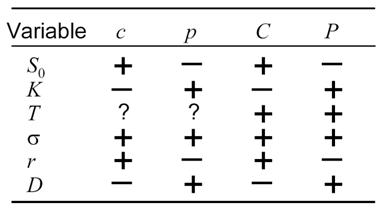
Systematic risks: the greeks

·  Delta (wrt price of the underlying asset)

o  Call: δ =e-qT N(d1)

o  Put: δ=-e-qT N(-d1)

·  Rho (wrt risk-free rate)

o  Call: ρ=XTe-rT N(d2)

o  Put: ρ=-XTe-rT N(-d2)

·  Vega (wrt volatility)

·  Theta (wrt time)

Hedging strategies

·  Delta-neutral

·  Gamma-neutral

·  Delta-rho-neutral

Swaps

·  Interest rate swap: exchange of fixed-rate and floating-rate interest payments for a fixed par value

o  Sensitive to interest rate risk

o  Pricing swap: via decomposition of PV(fixed coupons) and PV(forward rate coupons)

v  The market price of the floating-rate bond equals par after each coupon payment!

·  Currency swap: exchange of interest payments in different currencies

o  Sensitive to interest rate and currency risks

Lecture 3. Measuring volatility

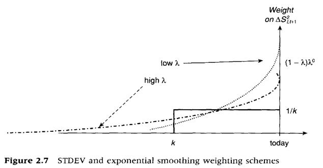
Historical volatility: MA

·  Moving Average with equal weights

EWMA (used by RiskMetrics)

σ2t = λσ2t-1 + (1-λ)r2t-1 = (1-λ) Σk>0 λt-1r2t-k

·  Exponentially Weighted Moving Average quickly absorbs shocks

·  λ is chosen to minimize Root of Mean Squared Error

RMSE = √ (1/T)∑t=1:T (σ2t-r2t)2

·  λ = 0.94 for developed markets

GARCH(1,1)

σ2t = a + b σ2t-1 + cε2t-1

·  Parameter restrictions: a>0, b+c<1

o  Guarantee that variation is non-negative and that unconditional expectation exists:
E[σ2] = a/(1-b-c)

·  More general model than EWMA, can be modified

o  More lags

o  Leverage effect: stronger reaction to negative shocks

·  More parameters leads to larger estimation error

o  Used less frequently in RM than EWMA

Implied

·  Based on options’ market prices and (Black-Sholes) model

o  Forward-looking!

Realized

·  Based on intraday data

o  E. g., prices over hourly intervals

o  Only for liquid assets

Lectures 4-7. Market risk: VaR and beyond

Identification of market risk

·  Primary: directional risks from taking a net long/short position in a given asset class

o  Interest rate / currency / equity / commodity

·  Secondary: other

o  Volatility / spread / dividend

o  Many trading books are managed with the objective of reducing primary risks…

v  at the expense of an increase in secondary risks

·  General (systematic) vs specific risks

o  The latter may be important because of lack of diversification or implementation of a specific investment strategy

·  Non-linear (option-like) instruments

o  Need to model full probability distribution of the underlying markets factor(s)

o  Sensitive to long-term market volatilities and correlations

Assessment of market risk: selection of factors and choice of models

·  Statistical models: factor return distributions

o  Describing uncertainty about the future values of market factors

o  E. g., geometric Brownian motion, GARCH

·  Pricing models: factor exposures

o  Relating the prices and sensitivities of instruments to underlying market factors

o  E. g., Black-Scholes

·  Risk aggregation models: risk measures

o  Evaluating the risk of losses in the future portfolio’s value

o  E. g., standard deviation, VaR

Traditional measures of market risk

·  Position

o  Size and direction

·  Volatility

o  Time aggregation: √T rule

o  Cross aggregation: diversification effect

·  Exposure

o  Stocks: beta

o  FI: duration, convexity

o  Derivatives: delta, gamma, vega, ...

Issues

·  Aggregation and comparability of risks

o  Can’t sum up deltas or vegas

o  Market vs credit vs operational risk

·  Measuring losses

·  Controlling risk: position limits

o  Until 1990s, mostly restrictions on size of net positions, including delta equivalent exposures

History of Market Risk Management

·  In late 1970s and 1980s,

o  Major financial institutions started work on internal models to measure and aggregate risks across the institution.

o  As firms became more complex, it was becoming more difficult but also more important to get a view of firm-wide risks

o  Firms lacked the methodology to aggregate risks from sub-firm level

·  Early 1990s

o  Group of 30 report. Derivatives: Practices and Principles. Their work helped shape the emerging field of financial risk management

o  Oct 1994 JP Morgan published RiskMetrics and made the data and methodology freely available on the internet. Riskmetrics was developed over the previous 8 months, based on their own internal model.

· 

o  Value at Risk (VaR) becomes a standard financial market risk measurement tool worldwide

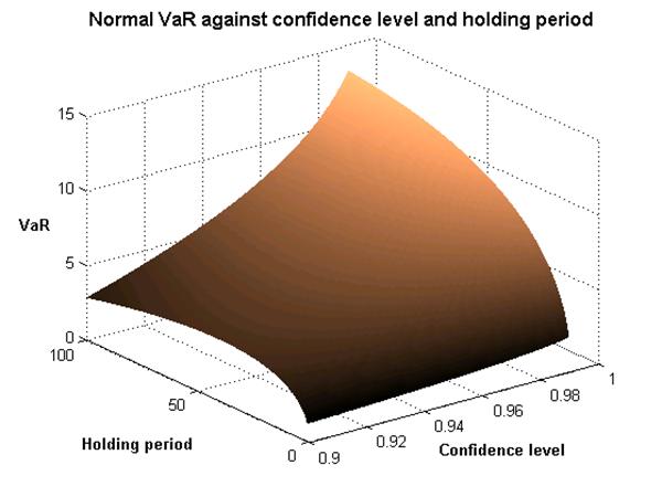
Value-at-Risk (VaR)

·  Maximum loss due to market fluctuations over a certain time period with a given probability 1-α:

Prob(Loss<VaR)=1-α

·  Key parameters:

o  Confidence level: 99% (Basel) or 95% (RiskMetrics)

v  The higher the confidence level, the lower the precision

o  Holding period: 10d (Basel) or 1d (RiskMetrics)

v  Time necessary to close or hedge the position

v  Investment horizon

·  Estimation period

·  Statistical model

VaR measurement: general framework

·  Marking-to-market position

·  Portfolio sensitivity to risk factors

o  Linear vs non-linear

·  Distribution of the risk factors

o  Normal vs other

·  Parameter assumptions

o  Confidence level and horizon

·  Data

o  Estimation period and frequency

Main methods of computing VaR

·  Delta-normal

o  Analytic, variance-covariance

·  Historical simulation

o  Bootstrap

·  Monte Carlo

o  Simulations

·  Stress Testing and Scenario Analysis are complementary tools to VaR

o  Focus on potential extreme market moves

Local estimation approaches

Standard delta-normal method

·  Assuming that ptf returns are normally distributed: VaR = V(1-exp(k1-ασt+μ)) ≈ k1-αVσt

o  Quantile: 1%) и 2%)

o  Daily data: assume that expected return = 0

·  Holding period up to 10 days

o  T-day Var = daily Var * √T

o  Assuming zero auto-correlation

·  Applications:

o  Single asset

o  Large, well-diversified ptf of many iid positions (e. g., consumer credits)

o  ‘Quick and dirty’ way to compute VaR of the business unit, based on historical P&L

Delta-normal method: risk mapping

·  Decomposition of the ptf to multiple risk factors: V = ΣiWiFi

VaR = k1-αV√WTΣW

o  V is decomposed based on Taylor series

o  W: vector of ptf weights or sensitivities of ptf return to factor returns

o  Σ: covariance matrix of risk factors

v  Can be decomposed to SD and correlations: covi, j = corri, j σi σj

v  Correlations are more stable in time, use larger estimation period

v  SD is more time-varying, computed by EWMA or GARCH

·  Decomposition of the ptf to standardized positions Xi

VaR = k1-α√XTΣX

o  Standardized positions: sensitive only to the given factor, with same delta as the ptf

v  Example: for a US investor, ptf of dollar bonds on $2 mln has std positions for interest rate risk on $2 mln and for FX risk on $2 mln

o  Two-stage approach by RiskMetrics: VaR = √ PVaRT Ω PVaR

v  Estimate risks of each std position: PVaR

v  Aggregate using pre-estimated correlation matrix of std positions Ω

Dealing with deviations from normal distribution:

·  Fat tails / skewness

o  Adjusted quantiles based on Student’s t distribution or mixture of normal distributions

·  Nonlinear relationships: dV = Δ dS + ½ Γ dS2 +Λ dσ + Θ dt + ...

o  Options: deltas are unstable and asymmetric

o  Delta-gamma-vega approximation: VaR = |Δ| k1-ασS – ½ Γ (k1-ασS)2 + |Λ| |dσ|

Critique

·  Quick computations

·  Decomposes risks

·  Strong assumptions about return distributions

·  Cannot handle complicated derivatives

·  The computations rise geometrically with # factors

·  Can’t aggregate volatility over time with √T for large T

Full estimation approaches

Historical simulation method: nonparametric, full estimation approach

·  Take historical time series of risk factors or assets

o  Usually, at least one year

o  Longer period increases the precision unless the process properties change over time

·  Simulate the change in value of a given ptf using historical factor realizations

o  Actual price functions (e. g., Black-Scholes)

o  Approximate ptf payoff function (based on ptf sensitivities)

·  Repeat simulations, plot the empirical distribution of P&L

Modifications:

·  Different probabilities for historical observations

o  EWMA: geometrically decreasing probabilities λt for lag t (0<λ<1)

v  More distant events have smaller probability

o  Higher weight for observations from the same month

v  For seasonal commodities, such as natural gas

·  Hull-White, standardized returns: use Ri, tsi/σi, t in the simulations

o  σi, t: historical volatility of factor i

o  si: current volatility forecast for factor i

·  Intra-day returns (e. g., hourly intervals)

o  Can analyze assets with short history (e. g., after IPO)

Critique

·  Easy and simple

·  No model risk

o  No need to assume normal distribution, forecast volatility

·  Correlations are embedded

·  Path-dependent, assumes stationarity

·  Requires long history

o  Otherwise miss rare shocks

·  Does not give structural knowledge

Monte Carlo (simulation) method

·  Model (multivariate) factor distributions

o  Stocks: Geometric Brownian Motion / with jumps

o  Interest rates: Vasicek / CIR / multifactor models

·  Generate scenarios and compute the realized P&L

o  Using factor innovations from the model

·  Plot the empirical distribution of P&L

Critique

·  Most powerful and flexible

o  (Cross-)factor dependencies

o  Most complicated instruments (path-dependent options)

·  Intellectual and technological skills required

·  Lengthy computations

·  Model risk

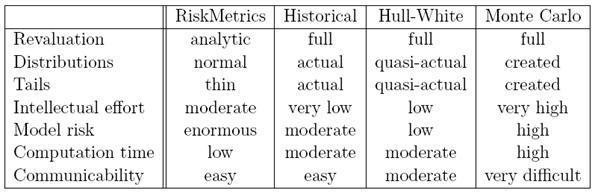
West (2004), Comparative summary of the methods

Different types of VaR

·  VaR delta: partial derivative wrt factor or position

·  VaR beta: % measuring the contribution of a given factor or position to the overall ptf risk

·  Incremental VaR: change in VaR due to a change in the position

o  Precise measurement requires re-estimation

·  Marginal (component) VaR: Delta*Position

o  Additive: ptf VaR is a sum of marginal VaRs

·  Relative VaR: VaR of the ptf’s deviation from the benchmark

o  Measures excessive risk

Backtesting VaR

·  Verification of how precisely VaR is measured

o  Compare % cases when the losses exceed VaR with the predicted frequency

·  Historical approach: based on the actual recorded P&L

o  More traditional, required by Basel

o  Helps to identify the model’s weaknesses, mistakes in the data, and intra-day trading

o  Often, actual P&L produces lower than expected frequency of VaR violations due to day trading that allows positions to be closed quickly when the markets become volatile

v  Thus, reducing actual losses compared holding a static portfolio for 24 hours

·  Hypothetical approach: based on hypothetical P&L computed using current ptf weights (factor exposures) and historical data on assets (risk factors)

o  Concentrates on the current risk profile

o  Eliminates the impact of intra-day trading

o  But: may give biased results if the same model is used both for estimating P&L and for VaR

·  Small sample problem

o  Need long history for high confidence level (99%) to ensure statistical accuracy of VaR

·  Basel: 1 year of daily data

# exceptions	Zone	Scaling factor for reserves
0-4	Green	3
5	Yellow	3.4
6	Yellow	3.5
7	Yellow	3.65
8	Yellow	3.75
9	Yellow	3.85
10+	Red	4 (model withdrawn)

Berkowitz and O’Brien, JF 2002

·  Examine the practice of VaR measurement in 6 large US banks

o  Compare VaR based on internal model with that based on reduced-form model for P&L

·  Data, 01/1998 – 03/2000

o  Consolidated end-of-day P&L, internal daily 99% VaR

o  The returns are normalized by SD to hide the identities of the banks

·  Т1: for 5 from 6 banks VaR is exceeded in 3 or less cases from 570

·  Т1, F1: when VaR is exceed, the losses are high, over 2 SD for 3 banks (prob. 0.1% for t5)

·  Т2, F2: most cases of exceeding VaR during the 3 months of the Russian default in 8-10/1998

o  Banks make conservative estimates of VaR: the exceptions are rare, but large and clustered in time

·  Т3: the correlation between banks’ daily P&L is quite low (0.2), the correlation between banks’ daily VaR is unstable

·  Т4: evaluating the accuracy of VaR estimates

o  Unconditional coverage test: reject H0 for one bank (but low power)

o  Independence (for i. i.d. distribution of violations): reject H0 for 2 banks

o  Conditional coverage test (sum of the previous two): reject H0 for 2 banks

·  Compare with the reduced-form models: ARMA(1,1) & GARCH(1,1), out-of-sample starting after 165 days

o  Does not account for change in positions and risks, cannot be used for sensitivity or scenario analysis

o  Embeds systematic mistakes in P&L

o  Т5, F4: VaR is lower, the average # exceptions close to 1%, the magnitude of losses is lower, similar test results

·  Conclusions:

o  Banks’ estimates of VaR are too conservative, do not adequately reflect risks in certain periods; are not better than those based on a simpler forecasting models (ARMA-GARCH)

o  Makes sense to use both models

v  Traditional: forward-looking, decomposes individual risks

v  Times series: flexible and parsimonious, advantage in forecasting, provides check for the main model

VaR implementation

·  Measurement

o  Local vs full estimation

o  Portfolio effects

·  Applications

·  Verification: back testing

·  Sensitivity: stress testing

·  Limitations

VaR applications

·  Portfolio management

o  Min VaR with given expected return

·  Position limits

o  Trading vs investment

o  Hierarchical structure

·  Capital adequacy requirements

o  Basel: reserves = 3*VaR99%

o  The multiplier goes up if VaR is underestimated

·  Risk-adjusted performance evaluation

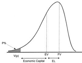
o  RAROC = Risk-Adjusted Return / Economic Capital

o  Similar measures in corporate finance: EaR (Earnings at Risk), CFaR (Cash Flow at Risk)

Stress testing

·  Analysis of ptf value under rare, but possible scenario

o  Shows the magnitude of losses which exceed VaR

o  Helps to identify the weaknesses

·  Factor push: assume that one of the key model parameters changes a lot

o  E. g., increase in volatility / correlations / exchange rate / oil price

o  For complicated derivatives need to check how the ptf value changes under different values of the parameter

o  But: correlations are ignored

·  Historical scenarios

o  August 1998: Russian gvt default, ruble devaluation, credit spreads rising, developed countries’ bonds rates falling, gradual liquidity crisis

o  Shock for a certain asset class: Black Monday for the US stock market in 1987, war in Iraq and oil price, etc.

o  Shock for a certain region: Asian crisis in 1997 (for emerging markets), USD weakening

o  9/11 terror attack, Enron reporting scandal, Yukos case, etc.

o  Advantage: keep correlation between different factors

·  Hypothetical scenarios

o  Rising correlations: e. g., model each asset’s return Ri as wtd sum of Ri & market return RM

o  Russia: bank crisis, inflation, WTO entry, …

o  It is important to ensure that there no internal inconsistencies in the perturbed model (e. g., arbitrage opportunities)

o  Advantage: very flexible

·  Hybrid method

o  Change the covariance matrix & other parameters

o  Estimate the conditional distribution of ptf value and compute ‘stress’ VaR

·  Extreme-value theory

o  Estimate the parameters of distribution of maximum losses

o  Block maxima: e. g., annual highest losses

o  Peak-over-threshold: 1% days with the lowest return

o  But: needs large and representative data base

Examples of scenarios

·  Stock market falling (e. g., US in 1987)

o  Developed stock markets falling by 20%, emerging ones by 30%; volatility rising by 25%

o  Flight to quality leads to strengthening of the dollar (by 10% relative to EM)

o  Interest rates in DM falling, EM % go up by 0.5% (1%) for long (short) maturities

o  Commodity prices falling due to fear of recession: oil price goes down by 5%

·  Tightening of the Fed’s monetary policy (to tighten up inflation, as in 1984)

o  Overnight rates rising by 1%, longer-maturity rates by 0.5%

o  Interest rates in other countries rising less

o  Relative strengthening of the dollar (investors put more in dollar-denominated instruments)

o  Credit spreads rising

o  Stock markets falling by 3-5%, volatility rising

Stress testing practice

·  Morgan Stanley: blue book

·  JP Morgan Chase: VID (vulnerability identification)

o  Re-estimation at least once a month, discussed by the top managers

o  Several macroeconomic crisis scenarios

o  Complementary scenarios for different market segments

o  Conservative assumption: positions remain the same during the crisis

v  To be ready to the abrupt fall in liquidity

·  Objective: be prepared to any possible financial crisis

o  Even though we don’t know its probability of occurring

RiskMetrics: JP Morgan & Reuters (since 1994)

·  Market risk measurement methodologies

o  Delta-normal / historical / Monte Carlo

o  Stress testing: VID (vulnerability identification)

·  Data on volatilities and correlations

o  Cash flow mapping to stock indices, currencies, and FI baskets

·  Software

Example: Orange County, $1.7 bln losses in 1994 due to rising %

·  Leveraged purchases of interest rate derivatives financed with reverse repos

o  Betting on the slope of the yield curve

·  Jorion: at the end of 1994, one-year 5% VaR was about $1 bln

o  Are the downside risks worth the upside?

o  Bad incentives for managers: either modest, above-market return or financial disaster

·  Miller and Ross: Orange County was not insolvent, with net assets of $6 bln, including $600 mln in cash (for $20 bln in total assets)

o  The bankruptcy could have easily been prevented!

Quiz

·  Total vs selective risk management

o  Value vs cash flow at risk

·  VaR vs expected return and upside potential

·  How to manipulate VaR?

·  What is the relation between Basel and RiskMetrics VaR?

·  Is it bad if the actual losses exceed VaR?

Beyond VaR

VaR assumptions

·  Portfolio sensitivity

o  Risk factor coverage

o  (Non-)linearity

·  Distributions

o  Stable and exploitable relationships

o  Fat tails and skewness

·  Arbitrary parameters

VaR drawbacks

·  Implicit assumptions

o  No intraday trading

o  Risks are described by exposures to several risk factors

o  Usually, second cross-derivatives are neglected

·  The actual losses are unknown

·  The measurement error may be large, esp. for a high confidence level

·  Model risk

·  Manipulation: incentive to choose

o  Strategies neutral to given risk factors

o  Portfolios with very unlikely extreme losses

·  Not subadditive

Properties of a coherent risk measure ρ

·  Monotonicity: ρ(X1) ≥ ρ(X2) for X1 ≤ X2

o  Higher return implies lower risk

·  Translation invariance: ρ(X+const) = ρ(X)-const

o  Adding cash lowers risk by the same amount

·  Homogeneity: ρ(λX) = λρ(X) for λ ≥ 0

o  Increasing the ptf’s size leads to proportional increase in risk

·  Subadditivity: ρ(X1+X2) ≤ ρ(X1) + ρ(X2)

o  Ptf risk does not exceed the sum of its components’ risks

Alternative market risk measures

·  Full distribution

·  Higher moments

o  Variance, kurtosis, etc.

·  Partial moments

o  Semi-variance: risks in the falling market

v  Downside CAPM: beta measured on the basis of low returns only

o  Expected shortfall (coherent!)

·  Cash flow risk

Lecture 8. Liquidity risk

Market liquidity: the ability to open or close large positions without a strong effect on price

Dimensions of market liquidity

·  Tightness: price deviation

o  Observed / Realized / Effective spread

v  Driven by inventory and adverse selection costs

·  Depth: potential supply and demand

o  Trading volume

o  Turnover rate (to volatility)

o  % non-traded days

o  Amihud (2002): daily ratio of absolute return to trading volume

v  Daily price response associated with $1 of trading

·  Resiliency: time necessary for price to recover

·  Immediacy: the execution time

Market microstructure estimates of illiquidity

The Glosten-Harris model: Δpt = λqt + ψ[Dt-Dt-1] + εt

·  Trade-by-trade data

·  D: order sign

o  Buyer (seller) initiated if the price is above (below) mid-quote: +1 (-1)

·  q: signed trade quantity

o  Positive for buyer-initiated trades

·  ψ: fixed cost component

·  λ: inverse market depth parameter

The Hasbrouck-Foster-Viswanathan model: Δpt = α + λqUt + ψ[Dt-Dt-1] + εt

·  qU: the unexpected signed trading volume

o  Based on the model for q with five lags of q and five lags of Δp

o  Measures the informativeness of trades

·  Cost components, in % of the price

o  Proportional: λ * avg trade size / avg closing price

o  Fixed: ψ / avg closing price

Liquidity and asset pricing

·  Lower transaction costs lead to lower equity premium for risk

·  Brennan (JFE, 1996):

o  Portfolios with higher estimated costs have higher expected return

v  Unexplained by Fama-French model

o  Higher spread implies lower returns!

v  Spread is a bad measure of illiquidity

·  Amihud (2002):

o  Expected illiquidity implies higher expected return

o  Unexpected decrease in liquidity decreases the current prices

Determinants of the liquidity

·  Asset characteristics

o  Substitution (leading to concentration) vs complementarity effects

·  Market microstructure

o  Transaction costs

o  Info transparency

o  Trading system

v  Auction vs dealership markets: price-volume trade-off

·  Behavioral factor

o  Dominating market participants

o  Heterogeneity

v  Buy/sell, risk attitude, investment horizon

Specifics of the Russian stock market

·  Liquidity is concentrated in blue chips

·  Liquidity moved from RTS to MICEX

·  Flight to liquidity (or quality) during the crises

o  E. g., August 1998, August 2003, April 2004

Modeling market liquidity risk

·  The actual price may differ from the current market price

·  The effective spread depends on the transaction size and timing

o  Harder to measure for the OTC market

o  Increases during the crisis

·  Monte Carlo analysis: VaR adjustment, accounting for

o  Direction and size of positions

v  No more positive homogeneity of degree 1

v  Ideally, should know elasticity of price wrt volume

o  Correlation between market dynamics and liquidity

v  Asymmetry between bullish and bearish markets

·  Stress testing, accounting for

o  Margin requirements

v  Esp. if you hold a large portfolio with one broker

o  Risk limits

v  Low limits will soon require further sales to stop losses

o  The likelihood of systemic crisis

o  Typical scenario: a dealer stops to provide quotes

Funding liquidity (insolvency) risk

·  Inability to fulfill the obligations because of the shortage of liquid funds

·  Determinants:

o  Current cash reserves

o  Ability to borrow or generate CFs

·  Sources:

o  Systemic

v  E. g., Russian gvt default in August 17, 1998

o  Individual

v  Change of a company’s (implicit) credit rating

o  Technical

v  Unbalanced forward payment structure

v  Uncertainty about future CFs

Example: LTCM

·  Investment strategy

o  Betting on convergence of spreads

v  E. g., long position on the off-the-run Treasury bonds, short position in the on-the-run (recently issued and more liquid) Treasuries

v  In general, long (short) position in riskier (less risky) instruments

o  High leverage, no diversification

o  Brought net returns over 40% in 1995 and 1996

o  But: sensitive to market-wide liquidity

·  At the end of 1997:

o  After returning $2.7 bln to their investors

o  Balance sheet assets of $125 bln

o  Off balance sheet notional amounts round $1 trln

v  Mostly nettable (swaps)

o  Positions with nominal value of $1.25 trln

·  Addressing funding liquidity risk:

o  Own capital of $4.8 bln

v  30 times leverage for BS sheet assets only!

o  Credit line of $900 mln

o  Investors commit capital for at least 2 years

·  The crisis and its resolution

o  August 1998: Russian default triggered “flight to safety”, all risk premiums rose

v  LTCM lost $550 mln in August 21 only

o  By the end of September, capital declined to $400 mln

v  LTCM was forced to liquidate positions to meet margin calls

o  September 1998: 90% of the LTCM ptf was purchased by a consortium of 14 banks for $3.625 bln

v  That prevented the danger that the default of LTCM would trigger many cross-defaults

o  July 1999: redemption of the fund

·  The issues raised

o  Risk management at LTCM

v  Role of stress testing

o  Risk management at LTCM counterparties

v  Interaction with a highly leveraged institution

o  Supervision

o  Moral hazard

Lectures 9-13. Credit risk

Credit risk: losses due to the counterparty’s failure to honour his obligations

Credit event

·  Default: an obligation is not honored

·  Payment default: an obligor does not make a payment when it is due

o  Repudiation: refusal to accept claim as valid

o  Moratorium: declaration to stop all payments for some period of time

v  Usually, by sovereigns

o  Credit default: payment default on borrowed money (loans and bonds)

·  Insolvency: inability to pay (even temporary)

·  Bankruptcy: the start of a formal legal procedure to ensure fair treatment of all creditors

Specifics of CR:

·  Asymmetry: possibility of big losses

o  “the most you can lose is everything”

·  Rare occurrence

·  Longer horizon

·  Non-tradability of most loans

o  Hard to measure correlations

·  Limits at the transaction level

·  Interaction with market risk

·  Esp important for banks

·  Larger reserves

o  Basel: 4*VaR

Examples

·  Savings&loans crisis in the US in 1980s

o  The restructuring cost the gvt $30 bln

·  Defaults on Latin American countries’ debt in 1980s

o  Restructuring in Brady bonds

·  Defaults on corporate bonds

o  Esp. junk bonds at the end of 1990s

·  Accumulation of bad quality loans in Japanese banks

·  Russia

o  No default on corporate bonds so far

o  Yukos on the brink of bankruptcy

Measuring credit risk

·  Basic components:

o  Probability of default (PD)

o  Recovery rate (RR) / loss given default (LGD), RR + LGD = 1

o  Credit exposure (CE) / Exposure at default (EAD), CE = EAD

·  Credit loss: CLi = Di*LGDi*EADi

o  Di: default indicator

·  The credit loss distribution: CL = Σi[Di*LGDi*EADi]

o  Highly skewed: limited upside, high downside

o  Correlation risk: assuming independence will underestimate risks

o  Concentration risk: sensitivity to the largest loans

·  Credit VaR = WCLα – E[CL]

o  Difference between expected losses and certain quantile of losses

o  Expected losses covered by ptf’s earnings

o  Unexpected losses covered by capital reserves

Modeling credit risk

·  Internal approach: usually used by banks, focus on PD

o  Classical solvency analysis

o  Market environment

o  Quality of the company’s management

o  Credit history

o  Credit product characteristics

·  External approach: using market data on stocks / bonds

MV(CR)= f(loss distribution, risk premium)

o  Need to measure both PD and RR

o  Requires liquid secondary market

Recovery rate

·  Highly variable, neglected by research for a long time

o  Fragmented and unreliable data

·  Market value recovery:

o  MV per unit of legal claim amount, short time (1/3m) after the default

·  Settlement value recovery:

o  Value of the default settlement per unit of legal claim amount, discounted back to the default date and after subtracting legal and administrative costs

·  Legal environment factors

o  Collateral or guarantees

o  Priority class: collateralized, senior, junior, etc.

o  The bankruptcy legislation

v  Large cross-country differences: e. g., US and France more obligor-friendly than UK

v  US bankruptcy procedures: ch. 11 (aim to restructure the obligor) vs ch. 7 (aim to liquidate the obligor and pay off debt)

·  Other empirically observed factors

o  Industry

o  The obligor’s rating prior to default

o  Business cycle & average rating in the industry

·  Altman: US,

o  On average, about 40% with SD of 20-30%

·  Modelling RR: beta distribution with density f(x) = c xa (1-x)b

o  For mean μ and variance σ2: a=μ2(1-μ)/σ2, b=μ(1-μ)2/σ2

Credit exposure: the amount we would lose in case of default with zero recovery

·  Only the positive economic value counts: current CEt=max(Vt, 0)

o  Vt: credit portfolio’s value

·  Current vs potential

o  Expected (ECE) vs Worst (WSE), for a given confidence level

·  Loans and bonds: direct, fixed exposures

o  Usually, at par

·  Commitments (e. g., line of credit): large potential exposure

o  Usually, fraction of par

·  OTC derivatives: variable exposures

o  Usually, at current value with adjustment for market risk

v  E. g., 90% quantile of the distribution

o  Interest rate swap:

v  Diffusion effect: increasing risk over time

v  Amortization effect: decreasing duration

Traditional approaches to CR measurement

Credit ratings

·  Independent agencies: S&P, Moody’s, Fitch

·  Integral estimate of the company’s solvency based on PD (and RR)

o  S&P: “general creditworthiness… based on relevant risk factors”

o  Moody’s: “future ability… of an issuer to make timely payments of principal and interest on a specific fixed-income security”

·  The rating procedure

o  Comprehensive analysis, from micro - to macro-level

v  Quantitative: based on financial reports

v  Qualitative: evaluation of the management (business perspectives, risk attitude, etc.)

v  Legal

o  The rating committee decides by voting

o  The rating is reconsidered at least once a year

·  Long-term company rating

o  Investment rating: from BBB (S&P), Baa (M’s)

v  Meant for conservative investors

o  Speculative rating

o  Smaller gradations: 1/2/3, +/-, Outlook, Watch

·  “Through-the-cycle” approach: CR at the worst point in cycle over contract’s maturity

o  Does not depend on the current market environment

o  In contrast to the “point-in-time” approach: CR depending on the current macro environment

·  Short-term company rating

·  Rating of specific instruments

Applications:

·  Credit policy and limits

·  Pricing the credit

·  Monitoring and credit control

·  Securitization

Survival analysis: actuarial approach to estimating PD

·  Sample period from 20 years

o  Need to accumulate default statistics (esp. for first-class issuers)

o  Need to account for different stages of the business cycles

·  For each rating: average PD

o  Equal weights: PD = # defaults / # companies (with a given rating)

v  Another approach: weights proportional to the issue’s volume

·  Type of the bonds

o  Bonds traded in the US market vs bonds of US companies

o  Straight bonds vs convertible/redeemable bonds

o  Newly issued bonds vs seasoned bonds

·  Horizon

o  Lower # observations for longer horizon

Measures of PD

·  Marginal mortality rate (MMR) in year t

o  Estimated PD in year t after the issuance

·  Survival rate (SR)

o  In year 1: SR1 = 1-MMR1

o  During T years: SRT = (1-MMR1)*…* (1-MMRT)

·  MR in year t given survival during t-1 years: MRt = SRt-1*MMRt

·  Cumulative MR during T years: CMRT = Σt=1:TMRt = 1-SRT

·  Average MR during T years: AMRT = 1-(1-CMRT)1/T

Estimation results

·  Cumulative PD goes down with rating

·  The highest MMR is for 4-5 years since the bond’s issuance

Critique of credit ratings

·  Ratings react with a lag to the change in the company’s solvency

·  Bias in ratings: too conservative

·  Large measurement error

o  Companies with the same (different) rating may have different (same) rating

o  Ratings of different agencies often do not coincide

·  Monte Carlo analysis by KMV

o  Generate 50,000 times a 25 year sample of N companies with a given PD

v  The parameters match those in Moody’s data base

o  The estimated PD is very noisy, higher than the actual one for most issuers

o  The differences between the estimated and actual PD rise with correlation between defaults

Credit ratings vs credit spreads

·  Credit spread of a given bond often differs from the avg in the group with the same credit rating

·  Credit spread depends on CR and other factors:

o  Liquidity risk

o  Maturity

o  Macroeconomic factors

o  Market volatility

·  Ratings react with a lag to the change in credit spread

o  Though the difference usually disappears with time: change in the firm’s solvency is reflected in rating within half a year, or spread returns to the initial value

Internal rating systems: evaluation of the borrower’s solvency

·  Criterions

o  Probability of default

o  Recovery rate

·  Horizon

o  Usually, 1 year

·  Scale

o  According to S&P/Moody’s or its own

·  Factors

o  E. g., 5C: Character, Capital, Capacity, Collateral, Cycle

Analysis of financial reports

·  Current / quick liquidity, leverage, profitability, turnover ratios

·  Backward-looking: using historical data

o  Extrapolation of the past into the future gives imprecise forecast

v  Esp. under high uncertainy

·  In Russia: little trust to fin reports

o  RAS is clearly inferior to IAS

o  Often reports are corrupted

v  To misguide tax authorities, minority shareholders, banks, etc.

Role of expert’s opinion

·  Visit to the company

·  Personal contact with opt managers

·  Human factor

Credit scoring models: predicting the default based on the borrower’s data

·  Altman’s Z-score (1968): linear function of 5 variables

o  X1: Working Capital to Assets

o  X2: Retained Earnings to Assets

o  X3: EBIT to Assets

o  X4: Market Value of Equity to Book Value of Liabilities

o  X5: Sales to Assets

·  The sample: 66 companies, half of which defaulted

Z = 1.2X1 + 1.4X2 + 3.3X3 + 0.6X4+ 0.999X5

·  Interpretation:

o  Z > 3: default is unlikely

o  2.7 < Z ≤ 3: closer to the “dangerous zone”

o  1.8 < Z ≤ 2.7: likely default

o  Z ≤ 1.8: very high PD

·  How to evaluate the model?

o  Type-1 error: default by the borrower who received a loan

o  Type-2 error: predicting default for the good borrower

o  Results: more than 90% firms were correctly classified

Constructing a scoring model

·  Financial variables:

o  Profitability, income volatility

o  Leverage and interest coverage

o  Liquidity

o  Capitalization

o  Management quality

·  Methodology

o  The binary choice logit / probit model

o  Discriminant analysis

·  Examples:

o  ZETA-model (1977): for big companies ($100 mln in assets)

v  7 variables instead of 5

o  EMS (emerging markets score): for emerging countries

v  Using the model calibrated by the US firms

v  Adjusted for the risk of currency’s devaluation, industry specifics, competitive advantage, presence of a guarantee, etc.

Critiqiue: pros and cons

·  Simplicity

·  Solves the problem of subjectivity of experts’ grades

·  Usually assumes simple linear dependence

·  Limited theory to explain the degree of each variable’s impact

o  Danger of overfitting in-sample

·  Need a good data-base

o  Usually, a biased sample excluding borrowers that were denied credit

·  Same old problems with financial report data

How to estimate losses of a credit portfolio?

Requirements to an ideal CR model

·  Instrument characteristics

o  Seniority

o  Collateral / guarantee

·  Company characteristics

o  Financial leverage

o  Balance liquidity

o  Type of the business: cyclical, growing

o  Size

·  Impact of macro factors

o  Recession

o  Decline in the stock or commodity market

o  Market liquidity crisis

·  Portfolio effects

o  Interaction between different credit instruments

o  Sensitivity to common risk factors

Basel requirements

·  The internal CR models should capture

o  Concentration / spread / downgrade / default risk

·  Capital charge = 4*VaR(99%, 10d)

·  Interaction between MR and CR

o  Spread risk includes both interest rate risk (MR) and default premium (CR)

o  Credit events are often anticipated and reflected in spread

o  Default is a special case of downgrade

·  Ideally: integrated approach to MR and CR measurement

Classification of CR models

·  Aggregation

o  Bottom up: start from individual positions

o  Top down: model aggregate credit portfolio

·  Type of CR

o  Default-mode (loss-based): an exposure is held till maturity, when it is repaid or defaults

o  Mark-to-market (NPV-based): track changes in the current market value of the instrument

·  Method of estimating PD:

o  Conditional: depending on the current stage of the business cycle

o  Unconditional

·  Modeling default

o  Structural: (endogenous) decision by the firm

o  Reduced-form: (exogenous) stochastic process

Proprietary models of credit risk

Benchmark CR models

·  CreditMetrics, 1997

o  JP Morgan Chase

·  KMV Portfolio Manager, 1998

o  Kealhofer, McQuown, Vasicek

·  CreditRisk+, 1997

o  Credit Suisse

·  Credit Portfolio View, 1997

o  McKinsey

CreditMetrics / Credit VaR I: CR driven by change in credit rating

·  CR is modeled as change in credit rating during a period equal to VaR horizon

o  Each rating is characterized by a certain PD

v  Assuming that all companies with same rating have same risk of default

o  Use migration probabilities (of moving from one to another rating)

o  Use data from one of the ratings agencies or internal ratings

·  Compute a probability distribution of the future value of the instrument, using

o  Forward rates for each rating

v  Thus, account for duration and spread effects

o  Recovery rate in case of default

v  Depending on seniority

·  Estimate VaR as a difference between a given quantile and expected value

·  Bottom up approach:

o  First estimate VaR for each instrument

o  Then aggregate to ptf VaR accounting for correlations

Migration of credit ratings

·  Transition matrix, usually for 1 year

o  Probability that a company with rating X next year receives rating Y

·  How to estimate T-year transition matrix?

o  Directly

v  But: increasing T means fewer observations and larger measurement error

o  Cross-multiplying annual transition matrices T times

v  But: ignoring auto-correlation effects

Example:

·  Bond with BBB rating, senior, unsecured, maturing in 5 years, 6% coupon rate

·  Ratings: S&P

o  7 groups: from AAA (first-class borrowers) to CCC (default)

·  Horizon: 1 year

o  Could be from 1 to 10 years

·  Annual forward curve for each rating

o  Allows us to compute the value of any bond in 1 year from now

Price of the bond in 1 year, if it keeps BBB rating

Forward distribution of the bond’s price

0.01 quantile of ΔV distribution: -23.91=VaR99%

CreditMetrics for a portfolio: diversification effect

·  Assume that return on assets is distributed as stock return (GBM)

·  Determine thresholds for the return distribution corresponding to the actual migration probabilities

·  Derive the correlation matrix

o  Based on multifactor model with user-defined country and industry weights

·  Monte Carlo analysis

o  Generate joint rating migration scenarios for bonds within the portfolio

o  Estimate the empirical distribution of ptf value and compute VaR

Critique

·  Ignore MR

o  Derivatives require stochastic interest rates

o  Esp. important to assume stochastic interest rates for derivatives

·  Assume homogeneity with the same rating class

·  Discrete migration matrix based on avg historical frequencies

o  Transition probabilities are usually underestimated

·  Simplified estimation procedure for correlations

Theoretical approaches to CR measurement

·  Structural approach: estimate risk-neutral PD

o  Use risky debt prices

o  Use equity prices and Merton (1974) option model

·  Reduced-form approach: use actuarial estimates of PD

o  Apply on the portfolio level

Credit spread analysis (based on bond’s market price)

·  For a one-period zero-coupon bond: r-rf ≈PD*LGD

o  LGD: relative to face value

·  Components:

o  Credit risk premium

v  Usually rising with maturity

o  Liquidity risk premium

·  Determinants:

o  Macro factors

v  Market volatility / liquidity

o  Bond characteristics

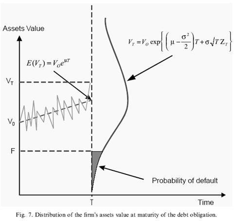
Merton model: stock as a call option on the value of the company V

·  Assume that V follows a log-normal distribution:

o  Zt~N(0,1): std Brownian motion

o  σV: volatility (SD) of the relative growth in V (dV/Vt)

o  μ: average growth rate, E[Vt]=V0eμt

·  The company’s capital structure includes

o  Equity, with value E

o  Debt (zero-coupon), with face value F and maturity T

·  Default occurs at maturity if VT<F

o  Stockholders receive at T: max(VT-F,0)

o  Creditors receive at T: min(VT, F)

·  Stockholders: call option on the value of the company V

o  Exercise date: T

o  Price of the underlying asset: V

o  Volatility: σV

·  Creditors: bond and short put

o  Or basic asset (the company) and short call

Derivation of the parameters:

·  V and σV are unobservable, derived from two equations:

o  The value of equity by Black-Scholes: E=V*N(d1)-Fe-rTN(d2)

v  r: risk-free rate

v  d1=[ln(V/F) + T(r+σ2/2)] / [σV√T], d2=d1-σV√T

o  The equation for stock volatility: σEE = N(d1) σVV

·  Risk-neutral probability of default: PD = 1-N(d2) = N(-d2)

·  Recovery rate (as % of the assets): RR = [1-N(d1)] / [1-N(d2)]

o  The current market value of debt: V-E=e-rT[(1-PD)+PD*RR]*F

Implicit assumptions:

·  Stockholders’ behavior – as given

o  Though they are interested in raising risk

·  Lognormal distribution

o  Underestimate PD at short horizon

·  Bankruptcy when V below the face value of debt

o  Default may be different from bankruptcy

KMV: main idea

·  Estimate PD using the modified Merton model

·  Move from empirical PD to risk-neutral PD

·  Derive analytically the future value of the company’s obligations and VaR

KMV Credit Monitor (1993): EDF model

·  Estimate the market value and volatility of the firm’s assets using modified Merton model

o  For public companies: estimate V and σV based on equity prices

v  Assume more complicated capital structure: equity, short-term debt, long-term debt, and convertible preferred shares

o  For private companies: estimate V and σV based on financial accounting measures

v  V is between the operational value (proportional to EBIT) and book value

v  σV is an empirical function of sales, assets, industry, etc.

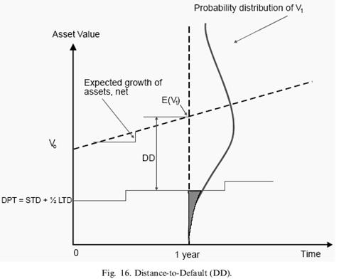
·  Compute distance to default (measure of default risk in T years)

o  Empirically estimated default point: DP = short-term liabilities + ½ long-term liabilities

o  Distance to default: DD = ln[E(V)-DP]/σV (in %, in σ)

·  Mapping DD to actual PD using historical data, for a given time horizon

o  Expected Default Frequency: EDF = # defaulted companies / # companies, for given DD

o  Can compute implied rating

Critique

·  Company-specific

·  Continuous, not biased by periods of high or low defaults

·  The correlation between defaults based on stock price correlations

·  Testing: EDF rises sharply 1-2 years before the default

o  Agencies’ ratings are slow to react

·  Best applied to publicly traded firms

o  Can’t estimate country risk

·  Ignore more complicated features of the debt

o  Seniority, collateral, etc.

KMV Portfolio Manager: CR driven by change in MV(assets)

·  Estimate actual EDF: KMV Credit Monitor

·  Derive risk-neutral EDF

o  Cumulative risk-neutral EDF at horizon T: QT = N[N-1(EDFT)+Sharpe√T)]

o  Substitute Sharpei=ρi*SharpeM*Tθ

v  In theory, θ=½

o  Calibrate the market Sharpe ratio and θ with observed corporate spreads over LIBOR

v  For maturity t: r-rf=(-1/t)ln(1-Q*LGD)

·  Estimate stock return correlation matrix using a 3-level multifactor model

o  Individual

o  Country and industry

o  Global and regional

·  Portfolio’s losses: L=VT(NoDefault)-VT(equilibrium)

o  Analytical derivation of VaR

o  The limiting loss distribution: normal inverse (highly skewed and leptokurtic)

Critique

·  Theoretically sound approach

o  Using risk-neutral probabilities

·  EDF is a good measure of default risk

·  Need market prices of equity

o  Assuming liquid market

o  Can’t estimate country risk

·  Hard to account for different types of debt

·  Behaviour of equityholders – as given

o  Though the have incentives and are able to increase risk

·  Assuming lognormal distribution

CreditRisk+: actuarial approach to estimate PD

·  Time horizon: usually, 1y

·  Assume

o  For each loan, PD is small and independent across periods

o  No assumption about the causes of the default

·  PD for a ptf: Poisson distribution, P(n defaults) = μnexp(-n)/n!

o  Avg # defaults: μ=ΣiPDi

o  St. dev.: √μ

·  Assume stochastical mean PD: μ is gamma-distributed

o  Otherwise, volatility of PD is underestimated

·  Exposure = Forward value * LGD

o  Differing exposure amounts may result in a loss distribution far from Poisson

·  The loan ptf is divided into exposure bands

o  Each band j has same exposure νj (in rounded units)

o  For each band, expected loss: εj=νjμjs

·  Deriving analytical distribution of ptf losses:

o  Probability generating function for each band

o  Probability generating function for the entire ptf

o  Loss distribution of the entire ptf

v  Depends on two sets of parameters: εj and νj

·  Extensions:

o  Hold-to-maturity horizon

v  Decompose the exposure profile over time

o  Multiple years

v  Take into account that default happens only once

o  Sector analysis: dealing with concentration risk

v  Assign sector-specific parameters to given obligors

o  Scenario analysis

·  Critique

o  Easy implementation

v  Focus on default

v  Few inputs

o  Analytical form of the results

o  Ignore MR and migration risk

o  Reduced-form

o  Not applicable to non-linear instruments

Credit Portfolio View: top down approach using macro factors

·  Assume PD(grade) = logistic f(macroeconomic index)

o  The index = linear f(macro and industry factors)

o  Each factor follows AR(2)

v  %, FX, industry growth

·  Estimate conditional rating migration matrix

o  Adjust the unconditional migration matrix by the ratio of conditional and unconditional simulated PD

o  Recession: more mass to downgrade migrations and PD

·  Monte Carlo analysis

o  Simulate the joint cond distribution of default and migration probabilities

·  Critique

o  Link macro factors to default and migration probabilities

o  Need reliable historical data on PD

o  Best applied to speculative grade obligors

o  Ad hoc procedure of estimating the migration matrix

Other models

·  CreditGrades: RiskMetrics, Goldman Sachs, JP Morgan, Deutche Bank

o  Stochastic default barrier: lognormally distributed, with possible discrete jumps

v  Increases estimated PD

o  PD is a closed form function of 6 parameters:

v  Mean and std of RR

v  Initial and current stock price

v  Implied stock volatility: calibrated from actual CDS spreads

o  CreditGrade = model implied 5y credit spread

·  Algorithmics Mark-to-Future (MtF): scenario-based approach

o  Links CR, MR, and LR

o  Generates cumulative PD conditional on scenario

Credit risk management

Impact of CR on derivatives

·  Derivatives on (credit) risky bonds

o  Long put gains in value

·  Vulnerable derivatives: subject to CR by the writer

o  The value diminishes by the credit spread: V’=V*Prisky(T)/PRF(T)

Traditional methods of CR management: credit exposure vs default modifiers

·  Modeling CE

o  BIS approach: CE = MV(deal) + potential CE

v  Usually, potential CE as 0-15% of par

o  Direct estimation of the potential CE distribution:

v  Stress-case / trees / Monte Carlo

·  Collateral arrangements: become popular for (longer-dated) swaps

o  Derivatives: usually, initial margin=0, variation margin only in case of MtM moves over the exposure limit

o  Longer period between remarkings

o  Post securities as collateral

·  Remarking / recouponing (to bring the value back to 0)

o  Usually quarterly

·  Netting: reduce potential CE to net position

o  Better assessed by scenario and simulation analysis

o  But: risk of “cherry-picking”

·  Credit guarantees

o  Esp valuable if the guarantee is from an independent company

o  Usually provided by parent companies

·  Credit triggers

o  Rating downgrade clause: right to terminate all transactions if the counterparty’s rating falls below the trigger level

·  Mutual termination option

o  Time put: right to terminate on one or more dates using a pre-agreed formula to value the transaction at these times

o  Termination brings CE to 0

·  Modeling recovery rate

o  Derivatives: usually, rank equally with senior unsecured debt

Implementation issues

·  Legal considerations

o  Collateral: maybe problems with enforceability in case of bankruptcy

·  Economic considerations

o  Resources required to implement recouponing and collateral arrangements

CR management instruments

·  Limits

o  Maturity / collateral / currency / regional / industry

·  Target levels

o  Return to CR

·  Diversification

·  Reserves

·  Credit derivatives

Credit derivatives

Evolution of derivatives: 3 waves

·  Second and third generation of price and event derivatives

o  Hybrid / contingent / path-dependent risks

·  Strategic management

o  Ptf risk, balance sheet growth, overall business performance

·  New underlying risks

o  Catastrophe / electricity / inflation / credit

Why credit derivatives?

·  Separate CR mgt from the underlying asset

o  Confidentiality

o  Customized terms

o  Objective and visible market pricing

·  Short-selling CR becomes possible

o  Arbitrage and efficient markets

·  Off-balance-sheet operations

o  Banks can avoid selling loans

§  Tax considerations / underpricing / client

o  Hedge funds can invest in CR, with leverage

§  Avoid transfer of property rights and administrative costs

·  Completing the market

o  Risk managers hedge CR

o  Issuers minimize liquidity costs

o  Investors find interesting instruments

·  Rapid growth since end of 1990s, currently over $2 trln

·  Types of insured CR:

o  Credit event, value of the underlying asset, recovery rate, maturity

·  Classified by:

o  Type of the underlying asset

o  Trigger event

o  Payoff function

Credit default swap:

·  Regular premium payments in exchange for a one-time premium in case of the credit event

o  Materiality clause: credit event is not triggered by a technical default

o  Both credit event and payments can be linked to a group of obligations

·  Settlement

o  Fixed payment

o  Cash settlement: difference between the strike (par) and current market price

o  Physical settlement in return of the par amount

·  Basket default swap

o  The underlying asset: loan portfolio

·  First-to-default (basket) swap

·  Dynamic credit swap

o  Changing principal

·  Practical role

o  Enhance liquidity

o  Hedging / investment opportunity

Total return swap:

·  Fixed or floating payments in exchange for the current income from the underlying asset

o  Regular exchange of payments

o  Insures both MR and CR

Credit options:

·  Call or put on the price of FRN, bond, loan, or asset swap package

o  (Multi-)European / American

o  Can knock out upon credit event

·  Practical role

o  Yield enhancement

o  Credit spread protection

o  Hedging future borrowing costs

·  Downgrade options

Other credit derivatives

·  Hybrid

o  Require a material movement in %, equity prices, …

·  Credit spread forwards / options

·  Credit-linked note: coupon payments conditional on the credit event

o  Usually via SPV (special purpose vehicle), trust company

Risks of credit derivatives

·  Correlation: simultaneous default of the underlying asset and protection seller

·  Basis

·  Legal

o  1999, 2003: ISDA adopted standard terms and documentation

·  Liquidity: usually traded OTC

·  Protection:

o  Bilateral netting

o  Option for premature abortion of the contract in the case of the counterparty’s financial distress

Lecture 14. Operational risk

Operational risk:

·  Definition 1: financial risks besides MR and CR

o  But: includes business risks

o  Did the credit default result from the ‘normal’ credit risk or mistake of the loan officer?

·  Definition 2: risks originating at financial transactions

o  But: excludes risks due to internal conflicts, model risk, …

·  Definition 3: risks due to deficiencies or mistakes from

o  Information systems and technologies

o  Internal procedures

o  Personnel

o  External events

Classification of OR

·  Operational failure (internal) risk

o  People: incompetency / fraud

o  Process: model / transaction / operating control risk

o  Technology: info systems, software, data bases

·  Operational strategic (external) risk

o  Environmental factors

o  Change in political and regulatory regime

·  Usually, business risk is excluded

o  Choice of strategy

o  Loss of reputation

o  Legal

Examples of OR failures

·  Barings and Nick Leeson (the “rogue trader”): more than $1 bln losses in 1995

o  Strategy: cash-futures arbitrage, Singapore-Osaka arbitrage

o  Booked losing trades to Account

o  End of 1992: hidden losses of 2 mln pounds

o  End of 1994: hidden losses of 208 mln pounds

o  1994: unauthorized positions in options

o  January 1995: earthquake in Kobe, massive margin calls

·  Daiwa bank and Iguchi Toshihide

o  Since 1979, VP in NY, average profit of $4mln

o  1984: loss of $50,000-200,000,

o  1996: losses accumulated to $1.1 bln, confessed

o  The bank hid this from Fed, was fined $340 mln and had to close its US operations

·  Sumitomo corporation and Hamanaka Yasuo, $2.6 bln total losses

o  Since 1975, in copper section, at heyday nicknamed “Mr. 5%”, “The Hammer”

o  From 1984: unauthorized speculative futures trading together with the head of the copper trading team, trying to boost profitability

o  1987: cumulative losses $58mln, Hamanaka became head of the copper section, received $150 mln from Merrill Lynch

o  1990: began borrowing money against Sumitomo’s trading stocks to fund his trading positions, started fictitious option trades to create an impression of success

o  1991: asked a broker to issue a backdated invoice for fictitious trades, worth $350 mln

§  The exchange notified Sumitomo, which replied it was needed for tax reasons

o  1993: borrowed $100 mln from ING using forged signatures of senior managers

o  1994: raised $150 mln from Morgan, then $350 mln from a 7-bank consortium

o  1995: investigations by US and UK regulators into unusual fluctuations in copper prices

o  March 1996: Sumitomo discovered that a statement from a foreign bank did not match its records

o  Hamanaka was jailed for 8 years, Sumitomo paid a fine of $150 mln in the US and $8 mln in the UK, Merrill Lynch paid a fine of $15 mln in the US and $10 mln in the UK,

o  Sumitomo filed suits against Morgan and other banks in assisting the illegal trades

Specifics of OR

·  Company-specific

·  Hard to quantify

·  Inverse relation between E(loss) and Prob(occurrence)

o  HFLS: high frequency, low severity

§  VaR techniques

o  LFHS: low frequency, high severity

§  Extreme value theory

·  Intentional (fraud) vs unintentional (mistakes)

·  Interaction with MR and CR

Quantification of OR: top down vs bottom up approaches

·  Indicators

o  Key performance indicators

§  E. g., # wrong operations

o  Key control indicators:

§  E. g., # prevented mistakes

o  Key risk indicators

§  Forecast OR based on performance and control indicators

·  Analysis of P&L volatility unexplained by MR and CR

·  Causal models

o  Measure losses using conditional probabilities

·  Distribution of P&L

Management of OR

·  Internal control system

o  General policy by top management

o  Assessment of risks

o  Control procedures

§  Internal: no conflicts of interests, double checking, approving access

§  External: confirmation, audit

o  Current monitoring

·  Financial transactions system

o  Front-office: “the face of the company”

o  Back-office: execution of the deals, accounting

o  Middle-office: input data, prepare papers, evaluate risks

·  Information system:

o  Data bases, software

o  Security, aggregation, interaction

New Basel agreement: reserves for OR

·  Basic indicator approach (BIA): ORC = αGI

o  GI: gross income, 3y avg

o  α: reservation coefficient, 15%

·  The standardized approach (TSA): ORC = Σi βi GIi

o  8 std directions: corporate finance, trading operations, payments (all 18%), retail (12%) and commercial banking (15%), intermediation (15%), asset management, brokerage (12%)

o  Alternative standardized approach: loans and advances instead of GI

·  Advanced measurement approaches (AMA)

o  Internal measurement approach (IMA): ORC = Σi γi ELi

§  Expected losses instead of GI based on PD, LGD, and correlations

§  Can be adjusted for risk profile index (RPI)

o  Loss distribution approach (LDA): ORC = Σi OVaRi

o  Scorecard approach

o  Up to 20% of OR exposure can be insured

Special risks

·  Model risk

o  Wrong model

o  Missing risk factor

o  Inputs

v  Low liquidity

·  Legal risk

o  Standardization

v  1992: ISDA Master agreement

·  Accounting risk

o  Marking-to-market

v  Low liquidity

o  Hedging vs speculative

o  Swaps

o  Taxation

Integrated risk-management

Recent developments

·  Increase in volatility after 1973

·  Globalization

·  Deregulation

·  Huge growth of the (exotic) derivatives market

·  Higher volume of the off-balance (derivatives) operations

·  Securitization

·  Technological progress

o  Electronic trading systems

o  Program trading

·  Conclusions:

o  Aggregation of risks

v  Importance of the enterprise-wide RM

v  Need unified framework

o  Higher systemic risks

o  Higher operational risks

RAROC (Bankers Trust, end of 70s)

·  Most popular risk-adjusted performance measure

o  Other: RORAC, RARORAC

·  RAROC = [Earnings – E(Loss)] / RC

o  Earnings: profit net of all taxes and expenses

o  Expected losses:

v  CR: f(PD, CE, RR)

v  MR: based on VaR models

o  Risk capital: reserves covering losses with given prob for given horizon

v  Can be adjusted with stress testing

·  Horizon: usually annual

o  Trade-off between MR and CR

·  Identification of risks

o  Usually: MR, CR, and OR

o  Additional: business, event, balance risks

·  Aggregation

o  Standard: RC = MRC + CRC + ORC

o  Monte Carlo

Applications of RAROC

·  Enterprise level:

o  Evaluate efficiency of work (backward-looking)

o  Optimal capital distribution (forward-looking)

o  Information for the outside world (shareholders, regulators, rating agencies)

o  Managerial compensation

·  Critique

o  Common bottom-up approach

o  Based on total risk (contrary to CAPM)

o  Inapplicable to risk-free instruments (unless impose positive reserves)

Regulation of banks

·  The standardized framework vs internal models

o  Internal models should satisfy certain criteria and be approved by CB

·  Basel Capital Accord (BIS I, 1988)

o  Differentiate the CR exposures

·  The 1995 amendment

o  Incorporate MR

·  The new Basel Capital Accord (BIS II, 2003)

o  Integrate MR, CR, and OR