Chapter 9 Risk analysis, real options, and capital budgeting (стр. 2 )

NPV= C0 + {[CSuccess (Prob. of Success)] + [CFailure (Prob. of Failure)]} / (1 + R)t

NPV = –$2,000,000 + {[$24,000,000 (0.75)] + [$6,000,000 (0.25)]} / 1.13

NPV = $15,256,637.17

The company should conduct the test marketing since that option has the highest expected payoff.

7. We need to calculate the NPV of each option, and choose the option with the highest NPV. So, the NPV of going directly to market is:

NPV = CSuccess (Prob. of Success)

NPV = $1,320,000 (0.50)

NPV = $660,000

The NPV of the focus group is:

NPV = C0 + CSuccess (Prob. of Success)

NPV = –$85,000 + $1,320,000 (0.70)

NPV = $839,000

And the NPV of using the consulting firm is:

NPV = C0 + CSuccess (Prob. of Success)

NPV = –$310,000 + $1,320,000 (0.90)

NPV = $878,000

The firm should hire the consulting firm since that option has the highest NPV.

8. The company should analyze both options, and choose the option with the greatest NPV. So, if the company goes to market immediately, the NPV is:

NPV = CSuccess (Prob. of Success) + CFailure (Prob. of Failure)

NPV = $28,000,000(.60) + $5,000,000(.40)

NPV = $18,800,000

Customer segment research requires a $750,000 cash outlay. Choosing the research option will also delay the launch of the product by one year. Thus, the expected payoff is delayed by one year and must be discounted back to year 0. So, the NPV of the customer segment research is:

NPV= C0 + {[CSuccess (Prob. of Success)] + [CFailure (Prob. of Failure)]} / (1 + R)t

NPV = –$750,000 + {[$28,000,000 (0.75)] + [$5,000,000 (0.25)]} / 1.12

NPV = $19,116,071.43

Graphically, the decision tree for the project is:

 

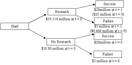The company should undertake the market segment research since it has the largest NPV.

9. a. The accounting breakeven is the aftertax sum of the fixed costs and depreciation charge divided by the aftertax contribution margin (selling price minus variable cost). So, the accounting breakeven level of sales is:

QA = [(FC + Depreciation)(1 – tC)] / [(P – VC)(1 – tC)]

QA = [($328,000 + $65,000) (1 – 0.35)] / [($3.75 – 0.84) (1 – 0.35)]

QA = 135,051.55

b. When calculating the financial breakeven point, we express the initial investment as an equivalent annual cost (EAC). Dividing the initial investment by the seven-year annuity factor, discounted at 13 percent, the EAC of the initial investment is:

EAC = Initial Investment / PVIFA13%,7

EAC = $455,000 / PVIFA13%,7

EAC = $102,880.42

Note that this calculation solves for the annuity payment with the initial investment as the present value of the annuity. In other words:

PVA = C({1 – [1/(1 + R)]t } / R)

$455,000 = C{[1 – (1/1.13)7 ] / .13}

C = $102,880.42

Now we can calculate the financial breakeven point. The financial breakeven point for this project is:

QF = [EAC + FC(1 – tC) – Depreciation(tC)] / [(P – VC)(1 – tC)]

QF = [$102,880.42 + $328,000(.65) – $65,000(.35)] / [($3.75 – 0.84) (.65)]

QF = 155,078.20

10. When calculating the financial breakeven point, we express the initial investment as an equivalent annual cost (EAC). Dividing the initial investment by the six-year annuity factor, discounted at 8 percent, the EAC of the initial investment is:

EAC = Initial Investment / PVIFA8%,65

EAC = $420,000 / PVIFA8%,6

EAC = $90,852.46

Note that this calculation solves for the annuity payment with the initial investment as the present value of the annuity. In other words:

PVA = C({1 – [1/(1 + R)]t } / R)

$420,000 = C{[1 – (1/1.08)6 ] / .08}

C = $90,852.46

The annual depreciation is the cost of the equipment divided by the economic life, or:

Annual depreciation = $420,000 / 6

Annual depreciation = $70,000

Now we can calculate the financial breakeven point. The financial breakeven point for this project is:

QF = [EAC + FC(1 – tC) – Depreciation(tC)] / [(P – VC)(1 – tC)]

QF = [$90,852.46 + $150,000(1 – .34) – $70,000(0.34)] / [($60 – 27) (1 – .34)]

QF = 7,624.08

Intermediate

11. a. At the accounting breakeven, the IRR is zero percent since the project recovers the initial investment. The payback period is N years, the length of the project since the initial investment is exactly recovered over the project life. The NPV at the accounting breakeven is:

NPV = I [(I/N)(PVIFAR%,N) – 1]

b. At the cash breakeven level, the IRR is –100 percent, the payback period is negative, and the NPV is negative and equal to the initial cash outlay.

c. The definition of the financial breakeven is where the NPV of the project is zero. If this is true, then the IRR of the project is equal to the required return. It is impossible to state the payback period, except to say that the payback period must be less than the length of the project. Since the discounted cash flows are equal to the initial investment, the undiscounted cash flows are greater than the initial investment, so the payback must be less than the project life.

12. Using the tax shield approach, the OCF at 83,000 units will be:

OCF = [(P – v)Q – FC](1 – tC) + tC(D)

OCF = [($31 – 17)(83,000) – 280,000](0.66) + 0.34($380,000/4)

OCF = $614,420

We will calculate the OCF at 84,000 units. The choice of the second level of quantity sold is arbitrary and irrelevant. No matter what level of units sold we choose, we will still get the same sensitivity. So, the OCF at this level of sales is:

OCF = [($31 – 17)(84,000) – 280,000](0.66) + 0.34($380,000/4)

OCF = $623,660

The sensitivity of the OCF to changes in the quantity sold is:

Sensitivity = DOCF/DQ = ($614,420 – 623,660)/(83,000 – 84,000)

DOCF/DQ = +$9.24

OCF will increase by $9.24 for every additional unit sold.

13. a. The base-case, best-case, and worst-case values are shown below. Remember that in the best-case, sales and price increase, while costs decrease. In the worst-case, sales and price decrease, and costs increase.

Scenario Unit sales Variable cost Fixed costs

Base 150 $15,300 $215,000

Best 165 $13,770 $193,500

Worst 135 $16,380 $236,500

Using the tax shield approach, the OCF and NPV for the base case estimate are:

OCFbase = [($19,500 – 15,300)(150) – $215,000](0.65) + 0.35($680,000/4)

OCFbase = $329,250

NPVbase = –$680,000 + $329,250(PVIFA15%,4)

NPVbase = $260,001.63

The OCF and NPV for the worst case estimate are:

OCFworst = [($19,500 – 16,830)(135) – $236,500](0.65) + 0.35($680,000/4)

OCFworst = $140,067.50

NPVworst = –$680,000 + $140,067.50(PVIFA15%,4)

NPVworst = –$280,110.32

And the OCF and NPV for the best case estimate are:

OCFbest = [($19,500 – 13,770)(165) – $193,500](0.65) + 0.35($680,000/4)

OCFbest = $548,267.50

NPVbest = –$680,000 + $548,267.50(PVIFA15%,4)

NPVbest = $885,291.85

b. To calculate the sensitivity of the NPV to changes in fixed costs, we choose another level of fixed costs. We will use fixed costs of $220,000. The OCF using this level of fixed costs and the other base case values with the tax shield approach, we get:

OCF = [($19,500 – 15,300)(150) – $220,000](0.65) + 0.35($380,000/4)

OCF = $326,000

And the NPV is:

NPV = –$680,000 + $326,000(PVIFA15%,4)

NPV = $250,772.95

The sensitivity of NPV to changes in fixed costs is:

DNPV/DFC = ($260,001.63 – 250,772.95)/($215,000 – 220,000)

DNPV/DFC = –$1.856

For every dollar FC increase, NPV falls by $1.86.

c. The accounting breakeven is:

QA = (FC + D)/(P – v)

QA = [$215,000 + ($680,000/4)]/($19,500 – 15,300)

QA = 91.67

14. The marketing study and the research and development are both sunk costs and should be ignored. We will calculate the sales and variable costs first. Since we will lose sales of the expensive clubs and gain sales of the cheap clubs, these must be accounted for as erosion. The total sales for the new project will be:

	Sales
	New clubs	$750 ´ 48,000 = $36,000,000
	Exp. clubs	$1,200 ´ (–13,000) = –15,600,000
	Cheap clubs	$420 ´ 10,000 = 4,200,000
		$24,600,000

For the variable costs, we must include the units gained or lost from the existing clubs. Note that the variable costs of the expensive clubs are an inflow. If we are not producing the sets any more, we will save these variable costs, which is an inflow. So:

	Var. costs
	New clubs	–$360 ´ 48,000 = –$17,280,000
	Exp. clubs	–$710 ´ (–13,000) = 9,230,000
	Cheap clubs	–$205 ´ 10,000 = –2,050,000
		–$10,100,000

The pro forma income statement will be:

	Sales	$24,600,000
	Variable costs	10,100,000
	Costs	7,500,000
	Depreciation	2,700,000
	EBT	4,300,000
	Taxes	1,720,000
	Net income	$ 2,580,000

Using the bottom up OCF calculation, we get:

OCF = NI + Depreciation = $2,580,000 + 2,700,000