

Партнерка на США и Канаду по недвижимости, выплаты в крипто
- 30% recurring commission
- Выплаты в USDT
- Вывод каждую неделю
- Комиссия до 5 лет за каждого referral
Требования к статьям, которые будут опубликованы в журналах, индексируемых в SCOPUS.
Язык – английский. Максимальное количество авторов: 3. Заглавие должно содержать не более 10 слов. Абстракт – 2 – 6 предложений (до 250 слов), отражающих вклад автора в исследование научной проблемы. Ключевые слова: 5 позиций. Просьба не использовать в ключевых словах общие термины, к примеру: “method”, “development”, “economics”. Размер текста: не более 5000 слов. Перед текстом статьи прикрепить сопроводительное письмо (см. приложение 4). В данном письме должны быть чётко отражены контактные данные автора, который будет ответственен за ведение переписки с редакцией журналов. Структура статьи может содержать следующие разделы: Introduction, Literature Review, Problem Statement and Research Objective, Key Results, Conclusions и Directions for further investigation, methodology description, hypotheses statement и др. Наличие расчётной части обязательно. Цитирование стандартное - APA referencing style. Для статей с единственным автором: (Sorderger, 2011) -, с несколькими: (Sorderger et al., 2013) – для официальных документов и файлов без авторов (The Law on Higher Education…, 1990). В исключительных случаях разрешаются прямые ссылки на интернет страницы, если они не слишком длинные. Таблицы и графический материал должны быть пронумерованы. В конце названия данных материалов должна быть дана ссылка на источник. Формулы должны быть пронумерованы. Весь графический материал должен быть высокого разрешения. Просим вас учесть, что журналы печатаются в чёрно – белой цветовой гамме. Для всех таблиц, графиков и рисунков необходимо наличие возможности редактировать их. Отсканированные материалы разрешены в исключительных случаях (в подавляющем большинстве случаев – карты). Благодарности и подстрочные сноски необходимо приводить в коне статьи. Не нумеруйте страницы. Надстрочные и подстрочные ссылки надписи использовать нельзя. Поля: 20 – верхнее и нижнее, 30 – левое, 10 – правое. Шрифт – Arial. Заголовок статьи: выравнивание по середине, жирный шрифт, 16pt. Названия разделов статьи: выравнивание по середине, жирный, 10pt, все буквы в названии – заглавные, пробел до и после названия раздела. Подзаголовки: 10pt, жирный, выравнивание по середине, пробел перед подзаголовком. Абстракт: 9pt, курсив. Основной текст: 10 pt, интервал после абзаца 6pt, 1,5 межстрочный интервал. Mathematics Subject classification смотреть здесь: http://www. ams. org/msc/msc2010.html . Journal of Economic Literature (JEL) Classification смотреть здесь: https://www. aeaweb. org/econlit/jelCodes. php? view=jel#Q Команда редакторов оставляет за собой право вносить незначительные изменения в текст, не влияющие на содержание работы. Мнение авторов статьи на проблемы политического и экономического характера может расходиться с мнением редакции журнала. Подробную информацию также можно просмотреть по следующей ссылке: http://www. ceser. in/ceserp/index. php/ijed/about/submissions#authorGuidelines Присылать статьи необходимо на почту: *****@***ru Образец оформления статьи ниже.
Example for Paper MS Word Template for the Journal: Models for the Prediction
A. Y. J. Akossou1 and R. Palm2
1Faculte d’Agronomie, Universite de Parakou,
BP 123, Parakou (Benin);
Email : *****@***com
2Faculte Universitaire des Sciences Agronomiques de Gembloux,
Avenue de la Faculte d’Agronomie, 8, B-5030 Gembloux (Belgique);
Email : *****@***com
ABSTRACT
Monte Carlo simulation method was used to study the effects of the data structure on the quality of the predictions in linear multiple regression. Five hundred forty (540) data files were generated of which the number of variables, R-square, the collinearity between the explanatory variables and the index of coefficient, that measures the importance of the explanatory variables in the model, were controlled. Predictions were influenced by the theoretical value of R-square, the method used to establish the model and, to a lesser extent, the collinearity between the explanatory variables. The determination of the minimal sample size which leads to predicted values better than those obtained by the mean of the dependent variable indicated that this size depends on the number of the explanatory variables, the theoretical value of the R-square and the method used to establish the model.
Keywords: Regression, data structure, prediction, simulation.
Mathematics Subject Classification: 62J12, 62G99
Journal of Economic Literature (JEL) Classification : Q12, D24
1. INTRODUCTION
In the establishment of the prediction model, three stages are fundamental: possible selection of the variables, the estimation of the coefficients of the variables selected and the validation of the model. Ideally, this validation should be done on different observations. But in most practical situations, the selection of the variables, the estimation of the coefficients and the validation are done using the same sample. Indeed, it is often difficult to have separate samples for the various stages of modeling, because the dataset available to the researcher is frequently too small to use part of it to establish the regression model and the remaining for its validation. Sometimes, the number of predictors is higher than the number of observations.
The objective of this work is to bring some useful information for the users, especially those who do not have the possibility to validate the models from external data. In a more concrete way, we propose to examine the predictive value of a regression model by calculating a coefficient, similar to the multiple coefficient of determination, which we call coefficient of determination of prediction. It is denoted ![]() and is defined, for
and is defined, for ![]() new observations, as follows:
new observations, as follows:
![]() .
.
In this relation, ![]() indicates the actual value of the dependent variable for the new individual
indicates the actual value of the dependent variable for the new individual ![]() (
(![]() ).
). ![]() , is the predicted value for this individual given by the regression model,
, is the predicted value for this individual given by the regression model, ![]() is the arithmetic mean of
is the arithmetic mean of ![]() observations of the dependent variable in the sample which was used to establish the model.
observations of the dependent variable in the sample which was used to establish the model.
2. GENERATION OF THE DATA
The realization of this work supposes the availability of a great number of repetitions of samples responding to the same known theoretical model. In practice, as the theoretical model is unknown, we use the Monte-Carlo method based on the generation of the data by computer according to a fixed theoretical model.
2.1. Theoretical model
We consider the traditional theoretical model of multiple linear regressions as:
![]()
where ![]() is an
is an ![]() vector observations of the dependent variables,
vector observations of the dependent variables, ![]() is the matrix
is the matrix ![]() of
of ![]() explanatory variable,
explanatory variable, ![]() the vector of
the vector of ![]() theoretical residuals and
theoretical residuals and ![]() the vector of the theoretical regression coefficients. It is supposed that the residuals are independent random variable of the same normal distribution of null mean and constant variance
the vector of the theoretical regression coefficients. It is supposed that the residuals are independent random variable of the same normal distribution of null mean and constant variance ![]() . The parameters to be simulated are
. The parameters to be simulated are ![]() ,
, ![]() and
and ![]() , while the vector
, while the vector ![]() is calculated by the model.
is calculated by the model.
2.2. Controlled factors
The factors controlled for the theoretical models are the number of explanatory variables ![]() , the number of observations (
, the number of observations (![]() ), the index of collinearity of the explanatory variables
), the index of collinearity of the explanatory variables ![]() , the index of decrease of the regression coefficients
, the index of decrease of the regression coefficients ![]() and the theoretical coefficient of determination
and the theoretical coefficient of determination ![]() .
.
![]()
where ![]() is the value of coefficient
is the value of coefficient ![]() ,
, ![]() the index of decrease of the regression coefficients and
the index of decrease of the regression coefficients and ![]() a constant.
a constant.
2.3. Methods of regression studied
On the one hand, we considered the classical method of least squares without variables selection and on the other hand, the stepwise selection method of variables is used. These methods were adopted, because they are among the most used methods, and are available in almost all statistical software.
The selection of variables is based on the t test of Student or F test of Snedecor for significance of the regression coefficients. We used the same level of significance for the introduction and the exclusion of a variable in the model. Two theoretical levels were retained: 0.15 and 0.05.
3. RESULTS
3.1. Effects of the various factors on the coefficient ![]()
The analysis of table 1 shows that coefficient ![]() is more often lower than the theoretical coefficient of determination. The ratio increases as the sample size increases, for a given value of
is more often lower than the theoretical coefficient of determination. The ratio increases as the sample size increases, for a given value of ![]() and
and ![]() .
.
Table 1: Average observed values of ![]() , expressed in proportion of
, expressed in proportion of ![]() , according to
, according to ![]() ,
, ![]() and
and ![]() .
.
|
|
|
|
|
|
Complete model | |||||
5 | 8 | -14.39 | -4.76 | -1.54 | 0.06 |
10 | 200 | 0.82 | 0.93 | 0.97 | 0.99 |
30 | 50 | -0.15 | 0.52 | 0.77 | 0.90 |
30 | 600 | 0.91 | 0.96 | 0.98 | 0.99 |
Model selected ( | |||||
30 | 600 | 0.93 | 1.00 | 1.00 | 1.00 |
For known values of ![]() and
and ![]() , the ratio
, the ratio ![]() /
/![]() depends little on the values of k and n. We also note that the ratio is weaker for the low values of
depends little on the values of k and n. We also note that the ratio is weaker for the low values of ![]() . Finally, the use of variables selection tends to increase the ratio.
. Finally, the use of variables selection tends to increase the ratio.
3.2. Determination of the levels of factors combinations leading to a null predictive value
In order to obtain results easily usable in practice, we determined the validity limits of the equations for the purpose of prediction by being unaware of the effect of factors ![]() and
and ![]() on the prediction. These limits are obtained by determining the levels of the ratio
on the prediction. These limits are obtained by determining the levels of the ratio ![]() leading to a zero value of
leading to a zero value of ![]() . These levels give on average the thresholds of combinations of factors from which the model led to predictions of quality lower than the prediction given by the arithmetic mean of the dependent variable of the sample.
. These levels give on average the thresholds of combinations of factors from which the model led to predictions of quality lower than the prediction given by the arithmetic mean of the dependent variable of the sample.
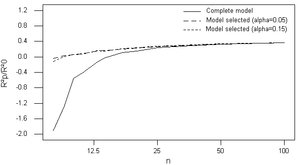
Figure 1. Evolution of the ratio ![]() /
/![]() according to the sample size on logarithmic scale in X-coordinate, for
according to the sample size on logarithmic scale in X-coordinate, for ![]() ,
, ![]() =0.40.
=0.40.
From this table, we note that this size varies according to the method used to establish the model. It is higher for the complete models and decreases gradually with the intensity of the selection. It also decreases as the theoretical value ![]() increases.
increases.
4. DISCUSSION AND CONCLUSION
Several authors documented criteria that assess the quality of a model. These criteria are based on the difference between the estimated model and the presumed known theoretical model. In the present study, the criterion used compares to new observations resulting from the same population as individuals of the sample, the variability of the errors of prediction, when the predictions are carried out by a regression equation and on the other hand when these predictions are equal to the arithmetic mean ![]() of the dependent variable in the sample. It thus gives an idea of the improvement of the quality of prediction by taking into account the explanatory variables. It also informs about the validity limits of a prediction model.
of the dependent variable in the sample. It thus gives an idea of the improvement of the quality of prediction by taking into account the explanatory variables. It also informs about the validity limits of a prediction model.
The plan of simulation considers data of varied structures. In particular, we considered the case where all the explanatory variables available are indeed present in the theoretical model (![]() ) and the case where certain explanatory variables available are not present in the theoretical model. This approach makes it possible to be close to the situations often encountered in practice.
) and the case where certain explanatory variables available are not present in the theoretical model. This approach makes it possible to be close to the situations often encountered in practice.
5. REFERENCES
Akossou, A. Y.J., 2005, Impact de la structure des donnees sur les predictions en regression lineaire multiple. PhD Thesis, Fac. Univ. Sci. Agron., Gembloux, Belgium, 215 p. Bendel, R. B., Afifi, A. A., 1977, Comparison of stopping rules in forward stepwise regression. J. Amer. Stat. Assoc. 72, 46-53.
Copas, R. D., 1983, Regression, prediction and shrinkage. J. R. Stat. Soc. B 45,311-354.
Dempster, A. P., Schatzoff, M., Wermuth N., 1977, A simulation study of alternatives to ordinary least squares. J. Amer. Stat. Assoc. 72, 77-106.
Meg, B. C., 1988, Determining the optimum number of predictors for linear prediction equation. Amer. Meteo. Soc. 116, 1623-1640.
Miller, A. J., 1990, Subset selection in regression. Monographs on statistics and applied probability 40. Chapman and Hall.
Palm, R., De Bast, A., Lahlou, M., 1991, Comparaison des modeles agrometeorologiques de type statistique empirique construits a partir de differents ensembles de variables meteorologiques. Bull. Rech. Agron. Gembloux 26, 71-89.
Roecker, E. B., 1991, Prediction error and its estimation for subset-selected models. Technometrics 33, 459-468.
