The investment strategies of publicly sponsored venture capital funds (стр. 7 )

We are particularly interested in obtaining from the model specific predictions concerning the distribution of the quality of the investments and their duration before the end of the investment cycle of the fund, as a function of the exit strategies undertaken. Indeed, scholars are often forced to measure such variables during the entire life of the fund, when good investments are more likely to be still active, while bad and short-term investments are over-represented in the sample of closed deals. In this case, the natural intuition that less patient investors will present a lower investment duration could be wrong.

Let us assume the investment of a certain quantity of capital – normalized to 1 – being the amount that must be employed for every investment.[12] The distribution of the return-factors (Ri) from one period investment is associated with three possible outcomes for the initial unitary investment – F, L and H – that represents, respectively, a case of write-off (RF = 0), a low (positive) return (RL), and a high return (RH), so that 1 < RL < RH. The investment lasts at most two periods. At the beginning (t = 0), the VC manager gathers information (i0) upon which it selects a firm from the population of available investment opportunities. At the end of the first period (t = 1), the VC receives a new signal about the characteristics of the target company. On the basis of this signal, the VC manager can decide to liquidate the investment at t = 1 or keep it in the portfolio for one additional period and sell the firm at t = 2. The VC fund can start a new investment round after the divestment in t = 1 or after selling the firm in t = 2. Let us define pH, pL, pF = 1 − pH − pL as the distribution (which is common knowledge) of the investment typologies in the population and πH, πL, πF = 1 − πH − πL as the subjective distribution in t = 0, which is updated by the VC manager given the signal i0, namely πk = prob (k|i0), with k = F, L, H. The quality of the information signal i0 depends on the selection capabilities of the investor. Obviously, all else being equal, the higher is pi , the higher will be πi.[13]

At time t = 1, the VC receives a second signal i1 that allows the information to be perfectly refined. Therefore, i1 assumes three values – f, l and h – that perfectly reveal the nature of the investment made in t = 0.[14] At time t = 1, the write-off signal f implies a compulsory liquidation of the assets, which as said generates null returns, while a signal equal to h implies to maintain the investment (no better firm can be found on the market). Only a signal equal to l can give rise to a discretionary choice between:

•  selling the company immediately for a value A > 0, after which it is possible to make a new round of investment, or

•  waiting one more period and obtaining R2L in t = 2.

We introduce now two additional simplifications that allow to easily compare the payoffs associated with the two alternative strategies of exit: i) the investment cycle of the VC fund has an indefinite duration and ii) after each divestment, the generated returns are distributed to the fund’s shareholders and the fund starts the collection (without additional costs) of a new unit of capital, that will give rise to a new round of investment.

Let us compare the payoff for the VC fund if it adopts the strategy consisting of divesting (D) in t = 1 when the signal is l (ΠD) and the strategy consisting of maintaining (M) the company in the portfolio when the signal is l (ΠM). The payoffs can be obtained in a recursive way thanks to the infinite life of the fund.[15] Given the discount factors δ requested by the VC shareholders under the two strategies,[16] it is possible to obtain the value of the fund in t = 0.

	(1)
	(2)

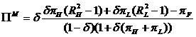
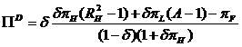
From the previous equations, we can derive the two expressions for the payoffs at time t = 0 in the case of strategy M and D:

From the above expressions, it is possible to obtain the internal rate of return (IRR) of the investment under the two strategies, given that the initial value of the investment is equal to 1.

	(3)
	(4)

Prediction of investment duration

As can be obtained by directly comparing eq. (3) and eq. (4), the prevalence of a “patient” (M) or “impatient” (D) strategy is not easy to understand, since it depends on several interacting variables. A more impatient strategy, which aims at divesting as soon as possible those investments of intermediate value in order to maximize the probability of getting a high return deal in the future, is more attractive when:

1. RH is high compared with RL;

2. πH is high compared with πL and πF is relatively low;

3. A is relatively high with respect to the expected proceeds at time t = 2.

In other words, investors will be impatient when they value the return of the high quality investments much more than the return of intermediate quality investments, when the offer of new ventures is favorable and when the proceeds that can be obtained on exit are high.[17]

Different characteristics of the two investment strategies, M or D, can then be derived. The funds that adopt the impatient strategy D should show a higher number of investments per unit of time. Accordingly, the expected duration of the investments is obviously different for the two strategies and equals τM = 1 + πH + πL and τD = 1 + πH, meaning that the average number of investments per unit of time is different. If one measures the duration of the investments after few investment rounds, however, no significant differences could be found since longer investments – more frequent when the M strategy is adopted – are still in place and their presence among closed deals results consequently lower.

Prediction of write-off frequency

The expected frequency of the investments of type H , L and F over a sufficiently long time horizon will be exactly equal to πH, πL, πF = 1 − πH − πL for both strategies, because every new investment is independently drawn – more or less frequently depending, respectively, on the adoption of a D or M strategy – from the same distribution.

Accordingly, those funds adopting an impatient strategy should show a higher number of investments per unit of time and therefore, comparatively, also a higher number of write-offs. The expected values for the number of defaults, conditional on the strategy, are in fact:

Nonetheless, as said, such a higher number of write-offs is associated with an identical frequency πF. Consequently, one should not expect a higher probability of default for the more impatient investors.

When funds are analyzed in a date before their expiration, the frequency of write-offs will result over-estimated, since in active deals longer and better investments are overrepresented. Since the D strategy presents a higher number of investments per unit of time, overestimation of write-offs which arises in the sub-sample of closed deals is likely to be, ceteris paribus, more relevant for patient investors. Nonetheless this is a second order effect, which can be reasonably neglected on empirical grounds.

ANNEX B – The duration models with year dummies

In this Annex we report the estimates for the duration models which also include year dummies.

Table B1 – Standard duration model and competing risk models. Dependent variable: duration of the investment. Coefficients reported.

	Duration model	Competing risk models
	Risk: any IRRs	Risk: IRR<0	Risk: -1<IRR<hurdle rate	Risk: 0<=IRR<hurdle rate
	Model I	Model II	Model III	Model IV
PUBLIC SHARE	-0.538***	-0.770***	-0.760***	-1.448**
	(0.163)	(0.222)	(0.262)	(0.593)
HIGHTECH	0.073	0.173*	0.086	0.256
	(0.070)	(0.091)	(0.115)	(0.266)
STARTUP	-0.096	0.300***	-0.089	-0.730***
	(0.062)	(0.080)	(0.100)	(0.225)
PATENTS	-0.577***	-0.808***	-0.562***	-0.119
	(0.075)	(0.096)	(0.114)	(0.233)
FUNDSIZE	-0.156***	-0.133**	-0.034	-0.212
	(0.040)	(0.053)	(0.063)	(0.143)
SEED FUND	0.103	0.461***	-0.075	-0.458
	(0.140)	(0.167)	(0.262)	(0.739)
INV PER	-0.030	0.002	1.038**	2.967***
	(0.247)	(0.415)	(0.465)	(0.950)
SME STOCK INDEX	0.250**	-0.737	-2.178**	-2.389
	(0.127)	(0.608)	(0.920)	(2.110)
Country dummies (fund)	Yes	Yes	Yes	Yes
Country dummies (company)	Yes	Yes	Yes	Yes
Year dummies	No	Yes	Yes	Yes
Observations	2482	2482	2482	2482
Failures	1288	796	511	107
Number of competing events	--	432	717	1121
Censored	1254	1254	1254	1254
LogLik	-2336.4	-5646.4	-3623.334	-734.418

Standard errors in parentheses. Significance levels: * 90%, ** 95%, *** 99%.