Потоки космических лучей в максимуме кривой поглощения в атмосфере и на границе атмосферы (1957–2007) (стр. 4 )

During 60ies the regular measurements of g-rays with energy Eg ³ 20 keV in the atmosphere of the northern polar and middle latitudes were made also. The standard radio sounds with NaJ(Tl) crystal as a g-ray detector was used. The crystal was of cylindrical form with diameter of 20 mm and length of 20 mm [6].

Treatment of experimental data has been made at Dolgoprudny scientific station of LPI RAS. A large amount of work was done by engineers, technicians, and laboratory assistants G. V. Yastrebtseva, A. F. Biryukova, K. A. Bogatskaya, A. M. Istratova, V. I. Obryvalova, G. V. Klishina, O. A. Shishkova, E. G. Plotnikova, G. I. Plugar, and many others.

In Table 1, the sites of regular measurements of charged particle and g-ray fluxes in the atmosphere are shown. The measurements have been done at the latitudes with different geomagnetic cutoff rigidities Rc and span the interval of altitudes from the ground level up to 30–35 km. At each level of measurements in the atmosphere the counting rate of detectors is defined by primary particles with rigidity above some cutoff value, so-called atmospheric cutoff rigidity Ra if Ra > Rc. Otherwise, if Ra < Rc, the cutoff is defined by geomagnetic cutoff rigidity Rc. For the data obtained with a single counter the dependence of Ra on atmospheric pressure is expressed as Ra = 4×10–2×x0.8 where Ra is in GV and х is in g×cm–2 [7].

Table 1. The sites and periods of measurements of CR and g-ray fluxes in the atmosphere

Site of measurements	Geographical coordinates	Rc, GV	Period of measurements
Loparskaya station, Olenya station, Apatity, Murmansk region	68°57¢N; 33°03¢E 67°33¢N; 33°20¢E	0. 6	07.1957–present time 03.1965–12.1968 (g)
Dolgoprudny, Moscow region	55°56¢N; 37°31¢E	2.4	07.1957–present time 10.1964–12.1969 (g)
Alma-Ata, Kazakhstan	43°15¢N; 76°55¢E	6.7	03.1962–04.1993
Mirny observatory, Antarctica	66°34¢S; 92°55¢E	0.03	03.1963–present time
Simeiz, Crimea	44°00¢N; 34°00¢E	5.9	03.1958–12.1961 03.1964–04.1970 10.1964–12.1969 (g)
Voyeikovo, Leningrad region	60°00¢N; 30°42¢E	1.7	11.1964–03.1970
Norilsk, Krasnoyarsk Territory	69°00¢N; 88°00¢E	0.6	11.1974–06.1982
Yerevan, Armenia	40°10¢N; 44°30¢E	7.6	01.1976–05.1989
Tixie, Yakutiya	71°36¢N; 128°54¢E	0.5	02.1978–09.1987
Dalnerechensk, Khabarovsk Territory	45°52¢N; 133°44¢E	7.35	08.1978–05.1982
Vostok station, Antarctica	78°47¢S; 106°87¢E	0.00	01.1980–02.1980
Barentzburg, Norway	78°36¢N; 16°24¢E	0.06	05.1982, 03–07.1983
Campinas, Brazil	23°00¢S; 47°08¢W	10.9	01.1988–02.1991

During the whole period of measurements, the identical detectors of charged particles (gas-discharged tubes of STS-6 type) and g-rays (NaJ(Tl) crystal) and identical devices for calibration of detectors have been used. Therefore, the sets of data given in Tables 3-32 are homogeneous.

The most long-lasting data series were obtained at the northern polar stations (Murmansk region) and at the midlatitude station (Dolgoprudny, Moscow region). These series span the period from the middle of 1957 up to now.

As an example in Figs. 1a, b monthly averaged counting rates of a single counter N1(x) and a telescope N2(x) at various latitudes are shown. The maxima in the counting rates N1m(x) and N2m(x) are distinctly seen. In comparison with the data obtained at other altitudes (N1(x) and N2(x)) the values of N1m and N2m have minimal statistical errors and do not depend on the accuracy of altitude or atmospheric pressure measurement. Fluxes of g-rays have similar dependence on the atmospheric pressure [6].

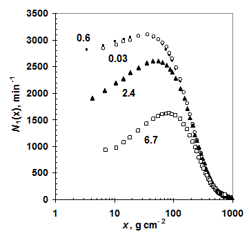
Fig. 1a. Monthly averaged counting rates of a single counter N1(x) vs. atmospheric pressure value x (absorption curves). The measurements were made during solar activity minimum in July 1987 at the northern polar latitude with the geomagnetic cutoff rigidity Rc = 0.6 GV (black circles), at the southern polar latitude with Rc = 0.03 GV (open circles), at the northern middle latitude with Rc = 2.4 GV (black triangles), and at the northern low latitude with Rc = 6.7 GV (open squares). The values of Rc are shown by figures near curves. The root-mean-square errors do not exceed sizes of the symbols.

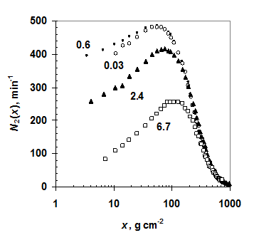
Fig. 1b. The same as in Fig. 1a but for data obtained with a telescope.

The following Tables 3–27 give the monthly averaged values of CR fluxes (galactic CRs and their secondaries in the atmosphere) measured with a single counter and a telescope in the maximum of absorption curve (N1m and N2m) with the root-mean-square errors s1 and s2 at the sites and for periods shown in Table 1. Tables 28–30 give the monthly averaged values of the g-rays fluxes of Ngm with energy Eg ³ 20 keV measured with crystal NaJ(Tl) in the maximum of absorption curve at the sites and for periods according to Table 1.

Determination of the particle fluxes at the atmospheric boundary

a) technique of extrapolation of particle flux values to the atmospheric boundary

From the altitude dependences of particle fluxes (see examples in Figs. 1a, b) one can find charged particle fluxes at the top of the atmosphere where atmospheric pressure х = 0. Let us take the differences between the counting rates at the latitudes with the geomagnetic cutoff rigidities Rc = 0.6 GV and Rc = 2.4 GV, as well as between Rc = 0.6 GV and Rc = 6.7 GV vs. residual pressure (or altitude) dN(x). For values of 4 < х £ 85 g×cm–2 these differences can be fitted to an exponential. As examples, in Figs. 2a, b and 3a, b these differences vs. х are plotted as obtained from the data presented in Figs. 1a, b for the solar activity minimum period (July 1987).

In Figs. 2a, b the approximation of differences obtained for a single counter and a telescope is shown together with the corresponding energy interval of primary protons (0.1 ≤ E ≤ 1.5 GeV). The logarithmic scale for the vertical axis is used. In Figs. 3a, b the differences for the second pair of altitude dependences (0.1 ≤ E ≤ 5.8 GeV) are shown. In this case the scale of both axes have linear and the differences are fitted to straight lines.

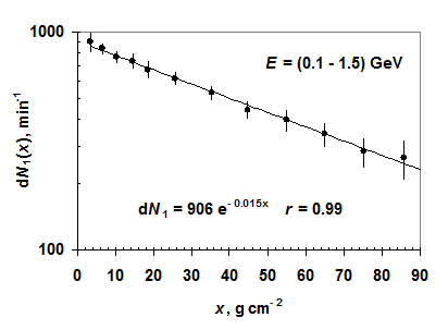
Fig. 2a. Differences dN1(х) between the counting rates of a single counter at the northern polar latitude (Rc = 0.6 GV) and that at the middle latitude (Rc = 2.4 GV) vs. atmospheric pressure х for the period of July 1987 (differences between the data of upper and middle absorption curves given in Fig. 1a). The scale of vertical axis is logarithmic. The vertical bars equal three root-mean-square errors (3s). The fitting law (see the figure) was calculated by the method of least squares, r – correlation coefficient between the experimental points and the approximation.

The approximating functions given at x = 0 yield the fluxes of charged particles at the top of the atmosphere (see examples in Figs. 2a, b and 3a, b). These fluxes include primary CRs J0 and secondary albedo particles JА. Subtracting the albedo particle flux JА from the values of charged particle fluxes at the top of the atmosphere yields the fluxes of primary CRs J0. The values of JA can be found in [8, 9]. An isotropic angular distribution of primary particles at the top of the atmosphere was assumed. In this case the geometrical factors Gcount = 16.4 сm2 for a single counter and Gtel = 17.8 сm2×sr for a telescope. Tables 31–32 give monthly averaged values of primary CR fluxes at the top of the atmosphere J0(Е ³ 0.1 GeV) and J0(0.1 £ Е £ 1.5 GeV).

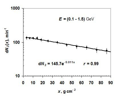
Fig. 2b. The same as in Fig. 2a but for the data obtained with a telescope at the northern polar latitude (Rc = 0.6 GV) and the northern middle latitude (Rc = 2.4 GV) for July 1987 (differences between the data of upper and middle absorption curves presented in Fig. 1b).

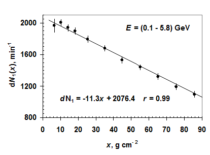
Fig. 3a. Differences of counting rates dN1(х) of a single counter at the northern polar latitude (Rc = 0.6 GV) and that at the northern low latitude (Rc = 6.7 GV) vs. atmospheric pressure х for the period of July 1987 (differences between the data of upper and bottom absorption curves given in Fig. 1a). The vertical bars equal three standard errors (3s). The straight line was calculated by the least-squares method, r – correlation coefficient between experimental and the fitting points.