Симулятор на основе сетей Петри для подготовки водителей (стр. 2 )

Overview of Petri Nets Approaches

According to the research task, for verification driver’s activity we are using Petri Net approach. There are different types and extensions of PN. We will observe the most suitable variants for applying them to the current task.

Classic Petri Nets

This is the basic type of PN. The definition of classic PN is formulated as (1):

A net is a triple N = (P, T, F) where - P is a set of places - T is a set of transitions, disjoint from P - F is a flow relation F ⊂ (P x T) ∪ (T x P) for the set of directed arcs.

(1)

PN can be represented as a directed bipartite graph. The state of the net is constituted by tokens in places. The tokens distributions in places are called markings. The holding of a condition is represented by a token in the corresponding place. A state can be performed by firing a transition. A transition “is enabled” or “can fire” if all its input places are marked by a token. Transition firing (the occurrence of a transition) means that all tokens are removed from the input places and are added to the output places. The transitions can fire concurrently or simultaneously – independently [4].

In general, we can apply this classical approach to the particular task. The main point is the way to reflect the real situation under the given model conditions. It is necessary to determined how traffic rules will be verifying through using Petri Nets. It is known that all drivers’ actions are recorded as the input values for the PN model. This model should have covering graph of all possible actions of the driver in case of the current street model. As a result the net can represent the rules that are applied to the road traffic way and also to the drivers’ behavior.

For the approach with classical PN we assume that state can be represented by two kind of usage. The first is the road parts and another state which contains the information about violation.

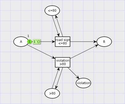
Fig. 1 Representation of thoroughfare with speed limit 80 km/h in terms of the classic PN model.

There is a simple example (Fig. 1) which contains the model of driving through the section of road with the limit in 80km/h. States A and B are parts of the highway where limit is currently in force. Token in A position is the representation of the car. In graphical real-time simulation the driver pass this section. He have the opportunity to change his speed during the transit. When he reaches the end the program analyses the maximum speed at this section. According to this result the executable state “>80” or “<=80” is marked. So, in case the speed was higher than limit state “>80” would contain the token. As a result the transition “violation >80” would be enabled. Its firing marks the “violation” state, which concludes that at this road section there was moving violation.

The model verifies the driver’s action according to its configuration. The PN should already contain all possible variants of situation respectively to the checking rules. The end result of verification is reflected on the specific states, which are known and created before simulations.

This method of modeling has some meaningful disadvantages. They can appear in more complex example (Fig. 2).

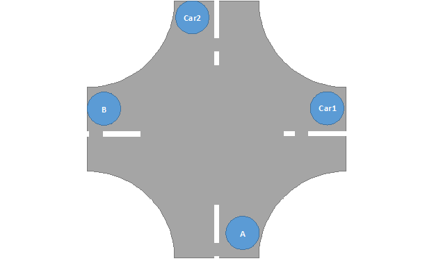
Fig. 2 Graphical representation of unregulated junction with oncoming traffic pointed as physical states of PN model.

According to the main examination factors from the Introduction part the most complex road situation is unregulated junction. Assumed that this cross of equal ranking roads. The exam task for the student-driver (A) is to turn left road (B) on the junction taking into account oncoming traffic (Car2) and traffic from the right road (Car1).

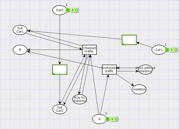
Fig. 3 Representation of unregulated junction with oncoming traffic in terms of the classic PN model.

In the PN model (Fig. 3) state A contains the start position of the student-driver’s car and according to the current task he should arrive to the state B. States Car1 and Car2 contains tokens which represent the existence of traffic on the up-to-down and right-to-left directions. The traffic will leave when all cars’ tokens will be in the end states Out Car1 and Out Car2 by firing the corresponding transitions. During simulation the program analyzes the driver’s behavior by the fact does he let pass or not. This property can be determined by stop the driver before crossing junction and monitoring locations of other cars in relatively driver’s point of view. All this factors are recorded in first come order. And when all traffic drive out, “Stop for checking” will be marked by the log and as a result “Checked traffic” transition can be fire. So there is no violation. Otherwise, the initial input state for the junction will be marked “Drive without checking” state. The result is rather intricate.

Also this model doesn’t considering the rules of using turning signals. At this case the model will be more complex. It means that we should add to all states witch are represented as sectors of the road new states and transitions with references to the conditions of turning signals. As a result, we consider that in each time we should check the drivers’ actions. Because it is necessary to supervise not only turning on the junction but also monitoring maneuverings on the highways’ lanes. Adding all this possible covering variants is a considerable overloading for the model. This leads us to the fact that implementing verification by using the model of classical PN is sufficiently limited and knotty.

The analysis shows that verification model is needed in separation of tokens’ type and in structure of street model driver’s behavior.

Colored Petri Nets

The first problem of tokens’ values separation can be solved by using the extended PN like Colored Petri Nets (CPN). At this net tokens distinguish by color or properties. The definition of CPN according to [5] is formulated as (2):

A CPN is a 5-tuple N = (P, T, C, W, m0), where - P is a set of places - T is a set of transitions, disjoint from P - C is the color-function defined from P∪ T into nonempty sets - W is the incident-function defined on P x T such that W(p, t)∈[C(t)→[C(p)→Z]] for all (p, t)∈ P x T - m0 is the initial marking, is function defined on P, such that m0 (p)∈[C(p)→N] for all p∈P.

(2)

In other words a token in CPN is represented as object with variables. Each state can contain only one type of the token. Depending on the arc function and condition transition execution is determined. Through transition execution the values of token can be changed. There is a simple example of using CPN in our task (Fig. 4).

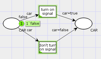
Fig. 4 Using token with Boolean property representing turning signals in terms of the CPN model.

There are two states with type of CAR which are the start and the end point of the turn road. The token of this type contains one value with Boolean type. In a particular example it can represent the information about turn signal. From the real-time simulation program store the condition of turn signal and then solves the relative CPN transition for this situation. After verification token would have the property referred to the rule violation.

Nevertheless this extension of PN doesn’t solve the problem with distinguishing drivers’ actions and structure of the road but only store in more convenient the violations and car properties.

Nested Petri Nets

Another problem with separating structure of street and car in PN model can be solved by using Nested Petri Nets (NPN) extension. NPN is extended CPN over a special universe. This universe consists of elements of some finite set S (called atomic tokens) and marked PN (called net tokens). For simplicity it’s considered here only two level NP nets, where net tokens are usual colored Petri nets over a finite universe [6]. The definition of NPN according to [7] is formulated as (3):

A NPN is a set N =(Atom, Lab, SN, (EN1 ,…, ENk), Λ), where - Atom = Var ∪ Con - is a set of atomic tokens - Lab = Labv ∪ Labh - is a set of markings - (EN1 ,…, ENk), (k ≥ 1) – is the finite set of classical PN (elements of NPN) - SN = (N, L, U, W, M0) – is a PN of high level, where o  N = (P, T, F) – is a net o  P – is a set of states with arity, P∩ Atom= ∅. o  L = Expr(Atom) – is a language of expressions o  U = (A, I) – is a model of language L, where A = Anet ∪ Aatom and Anet = {(EN, m) | ∃i =1,… , k : EN = ENi, m∈ M(ENi )},i. e., Anet – is a set of marking elementary nets. Set Anet is also the set of net tokens of the SN net. Set Aatom – is a finite set of atomic tokens. o  Function I: Con → A sets the particular interpretation of constants of language L. o  W – is a function which confronts to each arc (x, y)∈ F with a particular expression W (x, y) = (θ1 ,… , θn ) of n-dimension, where θi∈ L (1 ≤ i ≤ n) and n is the arity of the position with incident arc (x, y). o  M0 – is a dedicated marking (initial marking of the net) - Λ - is a partial function of transition marks, which marks some transitions of system nets by marks from Labv and some transitions of elementary nets by marks from Labv ∪ Labh.

(3)

In addition NP-nets can contain vertical and horizontal synchronization steps. A vertical synchronization includes simultaneous firing of transition, labeled with λ∈ Lab, in a system net together with firing of transitions, also labeled with λ in all net tokens involved in this system net transition firing [8]. A horizontal synchronization includes simultaneous firing of transition with the same labels of distinct elementary net tokens in one system place.